TraceWin
D. Uriot,
N. Pichoff, R. Duperrier
Université Paris-Saclay, CEA, Département des Accélérateurs, de la Cryogénie et du Magnétisme, 91191, Gif-sur-Yvette, France.
Updated, June 30, 2026
The TraceWin code calculates the beam dynamics in a particle accelerator. The beam is modelled both by its second-order momentum (fast computation, in linearised force) and/or by a macro-particle distribution (longer computation, in non-linear forces). Their simultaneous use makes it easy to study the influence of non-linear effects.
The different elements of a linac can be modelled either by analytical expressions or by field maps. The code is able to perform automatic procedures of accelerator and beam tuning, including statistical errors on elements and diagnostics.
TraceWin uses a very powerful GUI capable of providing a wide variety of plots. The user can modify any parameter and observe the effect very easily with the very powerful graphical display that allows visualising most of the useful parameters of the simulation (envelopes, beam ellipses, emittances, phase advances...). All this output can be easily saved to disk, saved in various image formats and inserted into reports (using copy and paste tools).
A large number of cases can be simulated remotely via a home-made client/server architecture. A heterogeneous array of machines can be used (Windows, Linux, MacOS). It is mainly written in C++ and Qt5.4 for Windows, Linux and MacOS operating systems. Started in 1998 (URIOT Didier and PICHOFF Nicolas), it is distributed under CEA licence since 2009.
Technical support & maintenance services
Using TraceWin in a batch command
Develop its own element or diagnostics
RF cavity transient analysis with TraceWin
CEA agrees to provide Licensee with updates and corrected versions of the Software. The content of Updates will be determined by CEA in its sole discretion and will include bug fixes, improvements and upgrades to bring the Software up to date with the latest version of the Software. However, Updates may not include: versions of the Software that are compatible with new operating systems, improvements, updates or new versions that are sold separately.
Updates and Corrected Versions shall be made available to Licensee in executable form by email in the manner specified by CEA.
CEA agrees to correct reproducible errors in the software programming. The Licensee shall notify CEA of any unidentified error and provide CEA with all information necessary to reproduce the error. The means used by CEA to correct an error will depend on the seriousness of the error.
If the error is due to a modification not made by or expressly authorised by CEA, the Licensee agrees to reimburse CEA for the time spent in correcting the error and restoring the Software to good working order, at CEA's rates in force at the time.
The CEA shall provide technical support to the Licensee during its normal office hours, Monday to Friday (excluding bank holidays and annual closing weeks). The CEA will use its best efforts to provide a detailed response within a maximum period of thirty (30) business days depending on the human resources available at the time of the request.
Requests should be sent to the CEA by e-mail to the contact address setout below. The Code can be downloaded at: http://irfu.cea.fr/Sacm/logiciels/ .
The CEA will add new features to the Software as required by a changes in the legal or regulatory requirements or in the software or hardware environment. New versions shall be made available to the Licensee, in executable form by e-mail in the manner specified by the CEA.
This version of TraceWin is maintained by Didier URIOT. We would appreciate to hear from you if you have a bug. You can send your questions or comments to the following emails address:
Very important: How to report a bug: Please use the button “Send project” on the main page and attach the specified files. In this way we will be able to know which system you are using and which version produced the bug and finally with the include files we can easily reproduce it and thus fix it
New: since December 2020, our communication policy regarding hotline, requests, bugs, help or more generally any question related to this software has evolved. We now offer an exchange via a dedicated forum: https://dacm-codes.fr/forum/
1 gigahertz (GHz) or faster 32-bit (x86) or 64-bit (x64) processor
1 gigabyte (GB) RAM (32-bit or 64-bit)
30 megabytes (MB) available hard drive space (32-bit or 64-bit)
Operating system:
Window (32-bit or-64-bit), version equal to or greater then WinXp
Linux (32-bit or-64-bit) with GLIBC library version equal to or greater than 2.6 (“ldd --version”)
MacOS with system version equal to or greater than 10.6
You're on a 64-bit system, you probably don’t have 32-bit library support installed. It’s mandatory for the defaut WebBrowser, QtWeb, internally used to get direct access to manual and also if want to use a 32bits TraceWin version.
To install (baseline) support for 32-bit executables
(if you don't use sudo in your setup read note below)
Most desktop Linux systems in the Fedora/Red Hat family:
pkcon install glibc.i686
Possibly some desktop Debian/Ubuntu systems:
pkcon install ia32-libs
Fedora or newer Red Hat, CentOS:
sudo dnf install glibc.i686
Older RHEL, CentOS:
sudo yum install glibc.i686
Even older RHEL, CentOS:
sudo yum install glibc.i386
Debian or Ubuntu:
sudo apt-get install ia32-libs
should grab you the (first, main) library you need.
Once you have that, you'll probably need support libs
Anyone needing to install glibc.i686 or glibc.i386 will probably run into other library dependencies, as well. To identify a package providing an arbitrary library, you can use
ldd /usr/bin/YOURAPPHERE
if you're not sure it's in /usr/bin you can also fall back on
ldd $(which YOURAPPNAME)
The output will look like this:
linux-gate.so.1 => (0xf7760000)
libpthread.so.0 => /lib/libpthread.so.0 (0xf773e000)
libSM.so.6 => not found
Check for missing libraries (e.g. libSM.so.6 in the above output), and for each one you need to find the package that provides it.
Commands to find the package per distribution family
Fedora/Red Hat Enterprise/CentOS:
dnf provides /usr/lib/libSM.so.6
or, on older RHEL/CentOS:
yum provides /usr/lib/libSM.so.6
or, on Debian/Ubuntu:
first, install and download the database for apt-file
sudo apt-get install apt-file && apt-file update
then search with
apt-file find libSM.so.6
Note the prefix path /usr/lib in the (usual) case; rarely, some libraries still live under /lib for historical reasons … On typical 64-bit systems, 32-bit libraries live in /usr/lib and 64-bit libraries live in /usr/lib64.
(Debian/Ubuntu organise multi-architecture libraries differently.)
Installing packages for missing libraries
The above should give you a package name, e.g.:
libSM-1.2.0-2.fc15.i686 : X.Org X11 SM runtime libraryRepo : fedoraMatched from:Filename : /usr/lib/libSM.so.6
In this example the name of the package is libSM and the name of the 32bit version of the package is libSM.i686.
You can then install the package to grab the requisite library using pkcon in a GUI, or sudo dnf/yum/apt-get as appropriate…. E.g pkcon install libSM.i686. If necessary you can specify the version fully. E.g sudo dnf install ibSM-1.2.0-2.fc15.i686.
Some libraries will have an “epoch” designator before their name; this can be omitted.
Warning
Incidentially, the issue you are facing either implies that your RPM (resp. DPkg/DSelect) database is corrupted, or that the application you're trying to run wasn't installed through the package manager. If you're new to Linux, you probably want to avoid using software from sources other than your package manager, whenever possible...
If you don't use "sudo" in your set-up
Type
su -c
every time you see sudo, eg,
su -c dnf install glibc.i686
No installation is required; all additional files used by TraceWin are extracted directly from the main code and installed when a process requires them.
The downloadable version is not a fully functional version. To activate its full capabilities, you must include a key file in the TraceWin executable directory: "tracewin.key".
Since TraceWin version 2.4.1.0 :
The activation key is generated automatically when the code is launched, when it is connected to the WEB and when the user is registered in the user database. To use the code on a computer without network access, you must bring this key file with the executable file to preserve the user rights.
Run the code directly by double-clicking the executable or the bundle for MacOS. To run from a batch command file, see the "Using the TraceWin batch command file" chapter.
· TraceWin is based in part on the work of the Qt project (http://qt.nokia.com) under the Qt Commercial Licence Agreement Version: 5.4
· TraceWin is partly based on the work of the Qwt project (http://qwt.sf.net).
· Documentation browser is provided by QtWeb, developed as a project of LogicWare & LSoft Technologies (http://qtweb.net/).
· A wide range of elements including RFQ with Toutatis module,
· 2D and 3D space charge,
· 1D, 2D and 3D static and RF magnetic and/or electric field maps (with superposition capability),
· Envelope simulation,
· macro-particle tracking simulations (number of particles depends on free memory),
· Each particle has a detailed analysis of its trajectory available,
· Start-to-finish simulations from source to target,
· transport of two beams in the same structure,
· and scattering analysis,
· Automatic transverse and longitudinal beam tuning in envelope and/or tracking mode,
· Beam tuning in period structure based on smoothing phase advances,
· Diagnostic-based correction procedures,
· Static and dynamic error simulations for all elements,
· Large particle number simulations for large scale calculations (Monte Carlo) based on client/server architecture,
· Statistical analysis including beam loss location,
· GUI and various auxiliary tools,
· Windows/Linux/MACOS versions,
· Reference code for the IFMIF, LINAC4, SPIRAL2, EUROTRANS, EURISOL and SPL projects.
TraceWin’s program is organized into 8 pages and 3 toolbars. These pages are described in more details below.
Menu : Displays the last 20 last projects currently open.
First toolBar : Open save or create a project file (configuration file, *.ini), display the currently open project.
Second toolBar : Start, pause or stop the process and set "auto_calculation".
Third toolBar : Visible only during matching, to stop or visualise the variation of the criteria.
Main page : To set input beam parameters, structure options and calculation options.
Multiparticle page : To configure multiparticle code options.
Matching page : To configure beam matching options
Output page : To visualise the calculation stages
Edit page : To modify or visualize the main input and output files.
Data page : To visualise the list of elements and commands from the data file
Charts page : To visualize the results with plots.
Errors page : To parameterise the error study and visualise results.
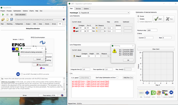
Epics page : To configure the EPICS virtual machine.
Each input or widget item of TraceWin GUI has an explanatory text. The default way for users to view the help is to move the focus to the relevant widget and press Shift+F1. The help text is displayed immediately. A second way is to use the Help button, see the following image.

TraceWin process is organized in several stages. The stages can automatically run one behind the other or not (“Auto calculation” button of ToolBar). Some of them can be disabled according to some options and commands.
|
|
|
|
Results saved |
Affected or used beam |
|
|
|
Stages
|
Required Conditions |
|
Main |
Second |
|
1 |
Read input data file and set tab in “Data” page |
|
|
|
|
|
2 |
Transport of the reference particle |
|
|
✔️ |
|
|
3 |
Set Phase advance law (set Quadrupole, Solenoid, Field map strengths) |
SET_ADV commands in data file or “Use file for phase adv definition” checked LATTICE commands in data file |
|
✔️ |
|
|
4 |
Read particle files |
Particle file defined in “Main” page |
|
✔️ |
✔️ |
|
5 |
Calculate the input matched beam |
“Calculate match beam” checked in “Matching” page |
|
✔️ |
✔️ |
|
6 |
Set quads or cavity strengths to match the beam through the different linac sections or set Twiss parameters (In order of theirs positions) |
“Matching with family” checked in page “Matching” MATCH_FAM commands and (LATTICE or SET_TWISS command) in data file |
✔️ |
✔️ |
|
|
7 |
Diagnostics (Example: Steerers) calculations (In the order of theirs numbers) |
“Match with diagnostics” checked in page “Matching” |
✔️ |
✔️ |
✔️ |
|
8 |
Input beam distribution (*.dst) is adjusted in order to fit the input beam defined in “Main” page or to fit the input matched beam calculated in (5) |
“Calculate match beam” -> “With partran” checked in “Matching” page “Use particle file” in “Input distribution type” in “Multipart” page Particle file defined in “Main” page |
|
|
|
|
9 |
Repetition of the preceding stages (5)(6)(7) using mutliparticle code |
On or several options “With partran” checked in “Match” page |
✔️ |
✔️ |
✔️ |
|
10 |
Random errors generator initialised |
“Reinitialize random generator” checked in “Main” page. |
|
|
|
|
11 |
Apply Static errors |
“Include error defined in…” checked in “Main” page “..Data No” in “Main” page set to errors defined in “Errors setup” of page “Error” “ERROR_xxx_STAT_xxxx” commands in data file |
|
✔️ |
✔️ |
|
12 |
Diagnostics (Example: Steerers) calculations |
“Match wiht diagnostics” in “Match” page Diagnostic elements and ADJUST commands in data file |
|
✔️ |
✔️ |
|
13 |
Repetition of the preceding stages (10 to 13) using mutliparticle code |
“Launch Partran” checked in “Multiparticle” page |
|
✔️ |
✔️ |
|
14 |
Apply dynamic errors |
“Include error defined in…” checked in “Main” page “..Data No” in “Main” page set to errors defined in “Errors setup” of page “Error” “ERROR_xxx_DYN_xxxx” commands in data file |
|
✔️ |
✔️ |
|
15 |
Calculates the transport line envelope |
Always |
|
✔️ |
✔️ |
|
Losses and beam parameters variations estimated in envelope transport |
“Nbr of particles” in “Main” page greater then 10 “Use aperture element” checked in “Main” page |
|
✔️ |
✔️ |
|
|
16 |
Write new data file in “calculation directory” |
Always |
|
|
|
|
17 |
Make the Error studies (envelope). N linacs, Loop with stage (10,11,12,14,15) |
“Study Envelope” checked in “Errors” page and error selection done |
|
✔️ |
✔️ |
|
18 |
Make the Error studies (Particles). N linacs, Loop with stage (10,11,12,13,14,15,19) |
“Study Multipartilce” checked in “Errors” page and error selection done |
|
✔️ |
✔️ |
|
19 |
Write input files of multiparticle codes PARTRAN and TOUTATIS and launch them |
“Launch Partran or Toutatis” checked in “Multiparticle” page |
|
✔️ |
✔️ |
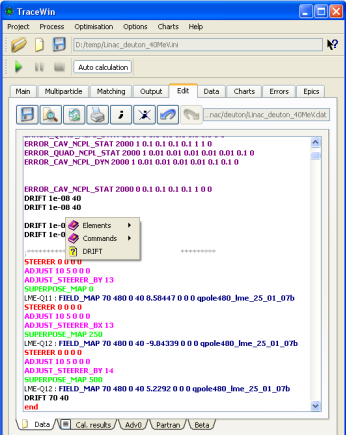
Some help on elements or commands in the data file editor can be obtained by using the right mouse button. If you don’t release it; the element number is displayed first.
Different king of plots, explore and test all the top buttons to well understand all the available options.
Zoom in by dragging a rectangle with the left mouse button.
Double-click the left mouse button to zoom out.
Move the plot area (only after zooming), with the right mouse button.
Save by
clicking on the appropriate icon ![]() in various image formats,
pdf, ps, data ASCII file.
in various image formats,
pdf, ps, data ASCII file.
Copy by
clicking on dedicated icon![]() in png format.
in png format.
Plot options,
colour, size, font, dots type… are configurable from icons ![]() .
.
All charts can be synchronised (refreshed after each calculation) by clicking on the dedicated icon.
The plot window can contain a maximum 6
plots using this icon ![]() .
.
For envelope plots, contextual information can be obtained by right clicking on any element; the envelope types (X, Y, X’, Y’, Z, Z’, Phase, Energy, Z, dp/p…) by right clicking on the plot.
For phase-space plots, the coordinates are selected by right clicking on the chart. In this case, you can either select one of the 8 proposed 2D phase-spaces or select the variable for each axis. It is possible to “Select” or “Unselect” the particles visible in the chart area. The sizes, colours of the selected or unselected particles can be configurated using the options button. This is very ususful for locating some particles in 6D phase-space and studing their behaviour in a line.
The emittance icon ![]() calculates and displays statistical information about the plotted
distribution. The code performs the same calculations for all plotted the phase-space
[x, y], whatever they are.
calculates and displays statistical information about the plotted
distribution. The code performs the same calculations for all plotted the phase-space
[x, y], whatever they are.
§
![]() ,
,
§
![]()
§
![]()
Emit [xx%] gives the ellipse surface, divided by p, homothetic to the rms ellipse, containing xx% of the beam particles. The xx is either the calculated fraction of particles within a homothetic ellipse whose area is N times the rms ellipse, or a given fraction of the beam. The plotted ellipses are the latter. The position of the c.o.g. and the size of the beam can also be calculated. Finally, two graphs can be plotted, the first showing the evolution of the number of particles outside a given emittance (scaled to the rms emittance calculated above), the second showing the evolution of the number of particles outside a given size (scaled to the rms size calculated above). The last button (s beam) shows the 6x6 beam matrix.
The emittances are calculated according to the “Energy and Phase limit” defined on the “Multipartcle” page.
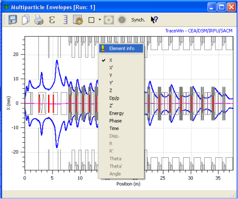
Envelope plot example
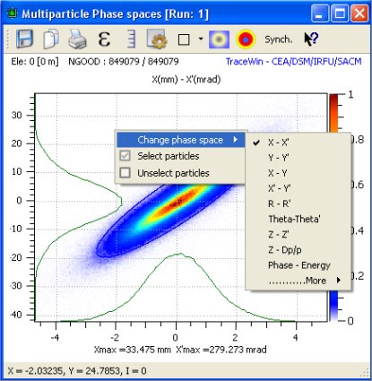
Multiparticle phase space plot
There are 3 ways to run TraceWIN in batch command corresponding to 3 types of executable files:
X11 or GUI full version
On an X console, hide the full TraceWin GUI / X11 with the “hide” command.
In this case, multi-threading and full code functionality is available, such as, for example, statistical error studies.
Syntax examples:
- For Linux or Mac:
./TraceWin /full_path/project_name.ini hide current1=80 freq1=352
- For Windows use a bat file and send the standard output to a file :
TraceWin d:\full_path\project_name.ini hide freq1=352 path_cal=c:\temp > output.txt
NoX11 or noGUI full version
On a command console:
- Linux executables: “./TraceWin64_noX11 ../projet_path/project.ini”
- Windows executables: “./TraceWin64_noGUI ../projet_path/project.ini”
- MacOS version could be suggested, if some users need them.
This executable is fully similar to GUI version except that no X11 / GUI is required. Multithreading and full error study on local and remote computers are also performed. The project configuration and file localisations must be exactly the same than for the GUI version. In other words, use the GUI version to configure your project or visualise results during an error study for example, but use the noX11 version to run the code if you need to exit the GUI during a process.
noX11 or noGUI minimal version
These versions are internally used by the main code for remote calculations performed during error studies. They are not available on the website but can be directly extracted using the top menu “Exe”.
On a command console:
- Windows executables: “tracew32.exe” & “tracew64.exe”
- Linux executables: “tracelx” & “tracelx64”
- MacOS executables: “tracemac” & “tracemac64”
In this case, multi-threading and statistical error studies are not possible. All project files must be located in the same directory as the executable file, so no path needs to be specified in the command line. Here, The “hide” argument means no standard output and the “hide_esc” argument means standard output without the ‘esc’ character.
Examples of syntax:
- For Linux or Mac:
./tracelx project_name.ini hide current1=80 freq1=352
- For Windows use bat file and send standard output to a file
Tracew32 project_name.ini freq1=352 current1=80
VARIABLE defned in structure file (*.dat) can be changed as argument.
For all the cases, the project file *.ini is automatically loaded. Input variables listed as arguments are modified. The calculation is started and TraceWin is closed at the end. The project name must be the first parameter and the input available variables are shown in the following tab. Input variables don’t need to be case-sensitive. The syntax is always “variable=value” without spaces, except for the “hide” variable. If the user needs another one, please, contact the developer.
The “tracewin.key” and possibly the “toutatis.key” must always be copied with the executable file.
In addition to these generic variables defined in the following table, the parameters of the element can be modified.
Examples of syntax for modifying element parameters:
tracew32 project_name.ini freq1=352 current1=80 Ele[15][2]=10
In this example, the second parameter of the 15th element will be set to 10. Respect the parameter units defined in the documentation for each element.
./tracelx64 project_name.ini freq1=352 current1=80 ele[15][2]=10 ele[25][3]=0.255
|
Ele[n][v] |
Change the vth parameter of for the nth element |
|
-version or -v |
TraceWin version |
|
hide |
Hide the GUI, or cancel console output (no parameter) |
|
tab_file |
Save to file the data page at the end of calcul (by default in calculation directory) |
|
upgrade |
Upgrade with last version available on CEA server |
|
Synoptic_file |
Save the geometric layout at (entance (=1), middle (=2), exit (=3) of elements. (See “Synoptic” tools for file name) . |
|
nbr_thread |
Set the max. number of core/thread used |
|
path_cal |
Calculation directory |
|
dat_file |
Full name of structure file |
|
dst_file1 |
Full name Input dst of main beam (*) |
|
dst_file2 |
Full name Input dst of second beam (*) |
|
current1 |
Input beam current (mA) of main beam |
|
current2 |
Input beam current (mA) of second beam |
|
nbr_part1 |
Number of particle of main beam |
|
nbr_part2 |
Number of particle of second beam |
|
energy1 |
Input kinetic energy (MeV) of main beam |
|
energy2 |
Input kinetic energy (MeV) of second beam |
|
etnx1 |
Input XX’ emittance (mm.mrad) of main beam |
|
etnx2 |
Input XX’ emittance (mm.mrad) of second beam |
|
etny1 |
Input YY’ emittance (mm.mrad) of main beam |
|
etny2 |
Input YY’ emittance (mm.mrad) of second beam |
|
eln1 |
Input ZZ’ emittance (mm.mrad) of main beam |
|
eln2 |
Input ZZ’ emittance (mm.mrad) of second beam |
|
freq1 |
Input beam frequency (MHz) of main beam |
|
freq2 |
Input beam frequency (MHz) of second beam |
|
duty1 |
Duty cycle of main beam |
|
duty2 |
Duty cycle of second beam |
|
mass1 |
Input beam mass (eV) of main beam
|
|
mass2 |
Input beam mass (eV) of second beam |
|
charge1 |
Input particle charge state of main beam |
|
charge2 |
Input particle charge state of second beam |
|
part_name1 |
Input particle charge state and mass of main beam |
|
part_name2 |
Input particle charge state and mass of second beam |
|
alpx1 |
Input twiss parameter alpXX’ of main beam |
|
alpx2 |
Input twiss parameter alpXX’ of second beam |
|
alpy1 |
Input twiss parameter alpYY’ of main beam |
|
alpy2 |
Input twiss parameter alpYY’ of second beam |
|
alpz1 |
Input twiss parameter alpZZ’ of main beam |
|
alpz2 |
Input twiss parameter alpZZ’ of second beam |
|
betx1 |
Input twiss parameter betXX’ of main beam |
|
betx2 |
Input twiss parameter betXX’ of second beam |
|
bety1 |
Input twiss parameter betYY’ of main beam |
|
bety2 |
Input twiss parameter betYY’ of second beam |
|
betz1 |
Input twiss parameter betZZ’ of main beam |
|
betz2 |
Input twiss parameter betZZ’ of second beam |
|
x1 |
Input X position of main beam |
|
x2 |
Input X position of second beam |
|
y1 |
Input Y position of main beam |
|
y2 |
Input Y position of second beam |
|
z1 |
Input Z position of main beam |
|
z2 |
Input Z position of second beam |
|
xp1 |
Input X angle of main beam |
|
xp2 |
Input X angle of second beam |
|
yp1 |
Input Y angle of main beam |
|
yp2 |
Input Y angle of second beam |
|
zp1 |
Input Z angle of main beam |
|
zp2 |
Input Z angle of second beam |
|
dw1 |
Input Dw of main beam |
|
dw2 |
Input Dw of second beam |
|
spreadw1 |
Input spread energy for DC beam of main beam |
|
spreadw2 |
Input spread energy for DC beam of second beam |
|
part_step |
Partran calculation step per meter (per beta.lambda if < 0) |
|
vfac |
Change RFQ Ucav (ex : “vfac 0.5”, half reduce of Ucav) |
|
random_seed |
Set the random seed |
|
partran |
Force or avoid tracking simulation (1 / 0) |
|
toutatis |
Force or avoid Toutatis simulation (1 / 0) |
|
algo |
Optimization using algorithm (0: Owner, 1: Simplex, 2: Diff. evo.) |
|
cancel_matcthing |
Cancel all matching procedure (Envelope) |
|
cancel_matcthingp |
Cancel all matching procedure (Tracking) |
|
picnir_2d |
Space-charge routine is defined as picnir2D |
|
picnic_3d |
Space-charge routine is defined as picnic3D |
|
picnir_r_mesh |
R mesh of picnir 2D |
|
picnir_z_mesh |
Z mesh of picnir 2D |
|
picnic_xy_mesh |
X&Y mesh of picnic 3D |
|
picnic_z_mesh |
Z mesh of picnic 3D |
|
input_dist_type |
Input distribution type from 1 to 5, see GUI menu |
|
use_dst_file |
dst file is used as input beam distribution |
|
trans_dist_mask |
Mask of the transverse input distribution from 1 to 7, see GUI menu |
|
long_dist_mask |
Mask of the longitudinal input distribution from 1 to 7, see GUI menu |
|
lost_e_limit |
Particle is lost if |W-Ws| > lost_e_limit |
|
lost_p_limit |
Particle is lost if |Ф- Ф s| > lost_p_limit |
|
emit_e_limit |
Particle is excluded form emit. calculation if |W-Ws|/ Ws > emit_e_limit |
|
emit_p_limit |
Particle is excluded form emit. calculation if |Ф- Ф s| > emit_p_limit |
|
back_tracking |
Transport tthe beam upside down through the machine |
(*): If the input dst file is specified, the input beam parameters (number of particles, emittances, Twiss parameters, beam centroid, beam current and energy) are automatically extracted from the specified file and used for the calculation. But you have to select the correct option "Use distribution from input particle file". The emittances and Twiss parameters cannot be modified by the corresponding input commands, but it is still possible to modify the beam centroid, current, energy and number of particles.
Step that allows to perform the calculation of the longitudinal acceptance on axis, zero current.
· Set the transverse emittances to a very small value (not zero).
· Set the longitudinal emittance and Twiss parameters in order to obtain a phase and energy spread greater than the expected acceptance of your structure.
· Set current to zero.
· Select uniform distribution.
· Set the number of particles to e.g. 10.000, for example.
· Set in “Multiparticle” page → “Distribution option file, PLT” option → “Last element” in order to avoid to generating a huge plt file size.
· Remove plt compression level.
· Remove in “Multiparticle” page → “Phase en energy limits” all condition (set everything to zero).
· Make a run in multipartcle mode (no matching have to be done here).
· In the “Chart” page, start “PlotWin” tool (if you don’t get it, upload it on the CEA site. This code must be started once for TraceWin to recognise it). Starting PlotWin from TraceWin allows to PlotWin to use the good PLT file directly, but you can also open the good one directly from PlotWin.
· In PlotWin, plot phase-space distribution of the last element of your structure. Here are only the surviving particles. If the number of particle is to small compared to your input beam, you probably have to reduce the phase or/and the energy spread of your input beam.
· Remove charts options such as “Losses” and “Create a 360° period”.
· Either select all the particles in the output distribution graph (left-click and "Select particles", as in the previous image) or, in most cases, it is preferable not to select the tails of particles that are too far from the expected reference energy.
· Now, in PlotWin, change the element number from the last one to 0, and plot the phase-space distribution again. The selected surviving particles should appear in a different colour. In the chart option (button at the top of the chart, you can choose the size, colour of the unselected and selected particles, you can also hide the unselected particles, in order to have only the input surviving particles).
· You visualise your longitudinal acceptance.
· In the ”Save” menu, you have the possibility of saving it (select “Particle checked”) in a dst file.
· You can, now, restart the whole step increasing the number of input particles in order to precisely define the acceptance (be careful, close PlotWin starting another process).
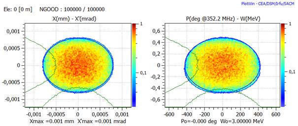
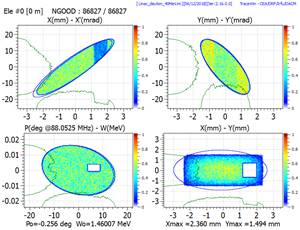
Input beam distribution at element 0, small in transverse and big in longitudinal
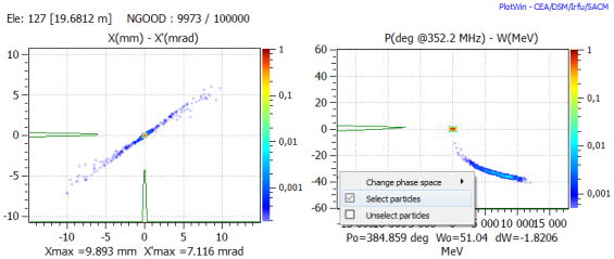
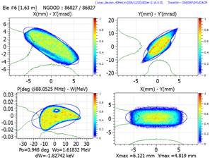
Surviving output distribution at last element (use menu to select all of them)
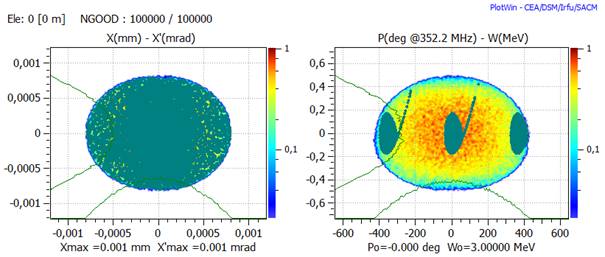
Input distribution at element 0, where acceptance is visible, here the space spread could be reduced.
PlotWin is a post-processing tool allowing to projecting and plotting a 6D beam distribution in 2D sub-phase-spaces and associated 1D beam density profiles. As many as 6 phase-spaces can be plotted on the same chart. The number of phase-spaces and the plot distribution can be selected. The beam is represented by a set of particles of equal weight. This tool allows each particle transport to be observed individually.
The code can be found at: http://irfu.cea.fr/Sacm/logiciels/
The beam density profile performed by TraceWin with the “Density” button is only a rough view of the beam density in R space. The aperture of the elements is divided into 100 rings, where the number of particles is counted in order to generate the density plot.
PlotWin provides much better quality density plots, as shown on in the following page.
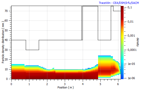
Distribution plot from TraceWin

The same distribution plot from PlotWin
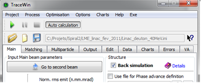
This option allows to transport a beam upside down through the machine from the end to the beginning. When the option “Back Simulation” is selected in the “Main” tab-sheet, the input beam has to be defined as the output beam of the machine. At the beginning of the run the structure of the machine is reversed (including the FIELD_MAP elements even superposed and other elements, accelerating or not). The space charge is also taken into account.
Two additional matrix elements are added at the beginning and end of the structure to apply the following changes to the beam.
![]()
L is the length of the elements.
For the FIELD_MAP elements specific case, two transformations are made:
![]()
And the name is change from “FIEL_MAP” to “MAP_FIELD” to make a clear distinction
A new structure file (*.dat ) is created corresponding to the reversed machine
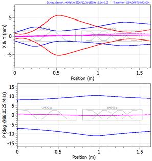
Example of reversed transport
The following example includes quadrupole and cavity field map:
SUPERPOSE_MAP 0
LME-Q11 : FIELD_MAP 70 480 0 40 9.174 0 0 0 qpole480_lme_25_01_07b
SUPERPOSE_MAP 250
LME-Q12 : FIELD_MAP 70 480 0 30 -7.4796 0 0 0 qpole480_lme_25_01_07b
DRIFT 70 40 0
SUPERPOSE_MAP 0
SET_SYNC_PHASE
LME-Gr1 : FIELD_MAP 7700 300 -20 30 0.33 0.33 0 0 carte_3gap_2b
SUPERPOSE_MAP 250
LME-Q13 : FIELD_MAP 70 480 0 40 2.784 0 0 0 qpole480_lme_25_01_07b
DRIFT 100 40 0
END
Once the run is finished,, we can find in the “Calculation” directory the new structure file corresponding to the back simulation done (bellow). Two THIN_MATRIX elements are there to reverse the beam and reverse back at the end, FIEL_MAP has been renamed to MAP_FIELD.
;------------------------------------
; ELEMENTS OF BACK TRACKING FILE
; ELEMENTS OF BACK TRACKING FILE
; 2 THIN_MATIRIX has been added at the beginning
; and at the end of the structure to reverse the
; beam for back transport
;------------------------------------
THIN_MATRIX 0 1 0 0 0 0 0 0 -1 0 0 0 0 0 0 1 0 0 0 0 0 0 -1 0 0 0 0 0 0 -1 0 0 0 0 0 0 1
DRIFT 100 40 0 0 0
SUPERPOSE_MAP 0 0 0 0 0 0
LME-Q13 : MAP_FIELD 70 480 0 40 2.784 0 0 0 qpole480_lme_25_01_07b
SET_SYNC_PHASE
SUPERPOSE_MAP 430 0 0 0 0 0
LME-Gr1 : MAP_FIELD 7700 300 -160 30 0.33 0.33 0 0 carte_3gap_2b
DRIFT 70 40 0 0 0
SUPERPOSE_MAP 0 0 0 0 0 0
LME-Q12 : MAP_FIELD 70 480 0 30 -7.4796 0 0 0 qpole480_lme_25_01_07b
SUPERPOSE_MAP 250 0 0 0 0 0
LME-Q11 : MAP_FIELD 70 480 0 40 9.174 0 0 0 qpole480_lme_25_01_07b
THIN_MATRIX 0 1 0 0 0 0 0 0 -1 0 0 0 0 0 0 1 0 0 0 0 0 0 -1 0 0 0 0 0 0 -1 0 0 0 0 0 0 1
END
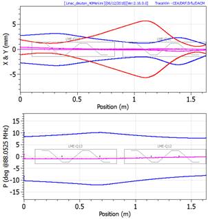
Normal transport results
Back simulation option is unchecked; this is the normal and usual beam transport.
|
|
|
|
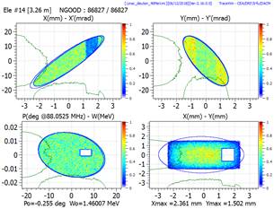
Input beam distribution. Holes are intentionally introduced into the transverse and longitudinal phase space. |
Output beam distribution |
|
|
|
|
Beam envelops. |
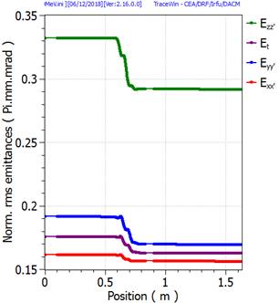
Emittances. |
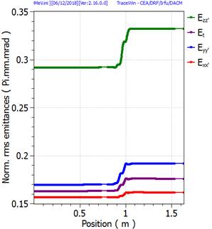
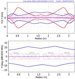
Back transport results
Back simulation option is checked and output beam distribution of preceding simulation is used as input beam
Another way consists to uncheck the “Back simulation” option and to use in normal simulation mode, the reversed structure file.
Both methods give the same results.
|
|
|
|
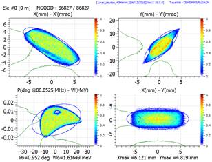
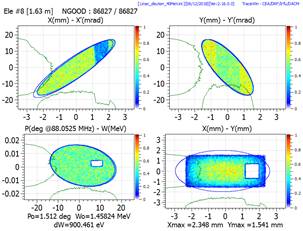
Input beam distribution |
Output beam distribution |
|
|
|
|
Beam envelops. |
Emittances. |
Checking reversed structure and code
Because reverse a structure could be a complex work and because it’s a nice way to verify this point and to check if the transport model (tracking or envelop) is consistent, it could be interesting to transport beam in the structure and in the reverse structure together. If every is good, you have to get output distribution identical to output one and also the transfer matrix of both structures has to be equal to the identity matrix. So considering the following structure file (Back simulation option unchecked)
SUPERPOSE_MAP 0
LME-Q11 : FIELD_MAP 70 480 0 40 9.174 0 0 0 qpole480_lme_25_01_07b
SUPERPOSE_MAP 250
LME-Q12 : FIELD_MAP 70 480 0 30 -7.4796 0 0 0 qpole480_lme_25_01_07b
DRIFT 70 40 0
SUPERPOSE_MAP 0
SET_SYNC_PHASE
LME-Gr1 : FIELD_MAP 7700 300 -20 30 0.33 0.33 0 0 carte_3gap_2b
SUPERPOSE_MAP 250
LME-Q13 : FIELD_MAP 70 480 0 40 2.784 0 0 0 qpole480_lme_25_01_07b
DRIFT 100 40 0
;------------------------------------
; ELEMENTS OF BACK TRACKING FILE
; ELEMENTS OF BACK TRACKING FILE
;------------------------------------
THIN_MATRIX 0 1 0 0 0 0 0 0 -1 0 0 0 0 0 0 1 0 0 0 0 0 0 -1 0 0 0 0 0 0 -1 0 0 0 0 0 0 1
DRIFT 100 40 0 0 0
SUPERPOSE_MAP 0 0 0 0 0 0
LME-Q13 : MAP_FIELD 70 480 0 40 2.784 0 0 0 qpole480_lme_25_01_07b
SET_SYNC_PHASE
SUPERPOSE_MAP 430 0 0 0 0 0
LME-Gr1 : MAP_FIELD 7700 300 -160 30 0.33 0.33 0 0 carte_3gap_2b
DRIFT 70 40 0 0 0
SUPERPOSE_MAP 0 0 0 0 0 0
LME-Q12 : MAP_FIELD 70 480 0 30 -7.4796 0 0 0 qpole480_lme_25_01_07b
SUPERPOSE_MAP 250 0 0 0 0 0
LME-Q11 : MAP_FIELD 70 480 0 40 9.174 0 0 0 qpole480_lme_25_01_07b
THIN_MATRIX 0 1 0 0 0 0 0 0 -1 0 0 0 0 0 0 1 0 0 0 0 0 0 -1 0 0 0 0 0 0 -1 0 0 0 0 0 0 1
END
Results
There is a perfect symmetry of the different beam parameters like output/input distributions, envelops and emittances.
|
|
|
|
Input beam distribution |
Output beam distribution |

|
|
|
|
Beam envelops. |
Emittances. |
Transfer matrix closed to be identical matrix, higher is the step of calculation, closer is this equality
Data file (*.dat)
Init project file (*.ini)
Results file (*.cal)
Adjusted value file (*.txt)
Steerer strength file (*.txt)
Cavity setting point file (*.txt)
Sigma0 file (*.sig0)
Input file for multiparticle program (*.par, *.dat)
Density file (*.dat)
Particle distribution (*.dat)
Lost particles (*.dat)
Error file results (*.txt)
Error set of data (*.txt)
Input & Output particle distribution (*.dst, *.plt)
Partran or Toutatis output (*.out)
Electric or magnetic field map
Current or space charge compensation map (*.scc)
Aperture map (*.ouv)
Magnetic stripping file (*.los)
Gas stripping file (*.los)
Random seed (*.log)
Transfer matrix (*.dat)
The data file ("*.dat") contains the list of elements and commands. It must be terminated with the "END" command. The syntax of the elements and commands is described in the "Element definitions" and "Command definitions" sections. The comment line starts with the ';' character.
A name of up to 50 characters can be specified for each element (see example below).
Result files are automatically created the first time the data file is used. At the end of a run, TraceWin creates another data file with the same name but located in the calculation directory and containing the new element list. For example, with the quadrupole values calculated to have the desired phase advance law. If the calculation directory is the same as the data file directory, the name of the new data file will begin with "new_...".
Warning:
Each command affects the following element, e.g. "SET_TWISS" will set some Twiss parameters at the output of the following element.
Two identical commands cannot follow each other.
; **********************************************
DRIFT 1e-08 100
SPACE_CHARGE_COMP 0.7
DRIFT 350 100
DRIFT 60 100
DRIFT 192 100
MATCH_FAM_GRAD 1 1
ADJUST 1 2 1 0 0
SOLENOID 410 0.25 100
DRIFT 100 100
MATCH_FAM_GRAD 1 2
STEERER 0 0 100 0
ADJUST_STEERER 2
ADJUST 1 2 2 0 0
QUAD 200 0.18 100 0
DRIFT 150 100
END
;**********************************************
; **********************************************
DR1 : DRIFT 1e-08 100
SP1 : SPACE_CHARGE_COMP 0.7
DR2 : DRIFT 350 100
DR3 : DRIFT 60 100
SOL 1 : SOLENOID 410 0.25 100
DR5 : DRIFT 100 100
QPF1 : QUAD 200 0.18 100 0
DR6 : DRIFT 150 100
;***********************************************
The init file “project_name.ini” contains all the TraceWin project parameters. It can be loaded, saved, copied by using the TraceWin menu.
It is created by TraceWin, its name is "Data_file_name.cal", it is located in the data file directory and it contains the results of the matching calculations already performed to avoid redundant calculations. See the following example.
Twiss_parameters_of_matched_beam
0.3167415265 0.1850852302 0.5246751875
-0.0938830920 0.0822867115 -0.0875778140
Matching_Between_Section_1_to_2
-8.11004 8.16711 -8.19803 8.21871
-3.8207 -2.8207 -4.1476 -1.1476
0.00834559 0.000887792
BEAM_FAM_69_0.DST
The first three lines are written after a matching beam calculation. The second line contains the Twiss parameters βxx', βyy', βzz' and the last αxx', αyy', αzz'.
The following five lines are written after a matching calculation, they contain the result of a matching between two sections. The first line contains the quadrupole gradients that have been adjusted ("MATCH_FAM_GRAD" command), the second line is either the phase shift or the field factor correction or both, of the accelerator elements that have been matched ("MATCH_FAM_PHASE", "MATCH_FAM_FIELD" or "MATCH_FAM_LFOC" command). The third line corresponds to the element length that has been adjusted ("MATCH_FAM_LENGTH" command) and the last is the name of a ray distribution file (located in the file data path) that will be saved when the matching family is calculated with the "With rays from Partran" option. All these lines are optional and depend on the "MATCH_FAM..." command in your data file.
For more details, see the matching commands and their examples. You can also force the optimisation of the calculation with initial values by using the following commands.
Init_Matching_Between_Section_1_to_2
-8.11004 8.16711 -8.19803 8.21871
-2.8207 -2.8207 -3.1476 -3.1476
To comment on a result, simply add the character ";" as the first character.
This file also contains all the diagnostic results, as in the following example. For more details, see the adjust commands and their examples. You can also force the optimisation process of the diagnostic calculation with initial values by using the "Init_" syntax.
Diagnostic_10
10.7992 -10.5893 5.81701
Init_Diagnostic_10
10.7992 -10.5893 5.81701
For all these result, an extension “_PAR” is added when the result comes from a multiparticle optimization ‘With Partran” is checked
Created by TraceWin or No, its name is "*.sig". It's located in the data file directory and contains the transverse phase advance law without current, one value per lattice. See the example below, where the red values correspond to the optional vertical phase advance, sigy=sigx by default.
60 40
60 41
61 41
62 42
…
..
.
Input field for “FIELD_MAP” element, see also FIELD_MAP details.
In “Chart” page a tool allows the visualization (1D or 2D) the field maps from elements defined in data file. This tool also allows to convert the field ASCII format to binary format. This allows the code to be faster if the size of the field maps is too large.
The field map file syntax in ASCII format is as follows:
Fz are in MV/m for electric field or in T for magnetic field.
For specific 3D aperture field map file, Fz = 0 or 1, 1 corresponding to material.
The dimensions are in metres.
- Dimension 1 :
Pay attention, to the number of data requested, N=(nz+1)
nz zmax
Norm
for k=0 to nz
Fz(k.zmax/nz)
Return
- Dimension 2 :
Pay attention, to the number of data requested, N=(nz+1)*(nr+1)
nz zmax
nr rmax
Norm
for k=0 to nz
for i=0 to nr
Fz(k×zmax/nz, i×rmax/nr)
Return
or
Pay attention, to the number of data requested, N=(nx+1)*ny+1)
nx xmin xmax
ny ymin ymax
Norm
for k=0 to ny
for i=0 to nx
Fz(k×xmax/nx, i×ymax/ny)
Return
- Dimension 3 :
nz zmax
nx xmin xmax
ny ymin ymax
Norm
for k=0 to nz
for j=0 to ny
for i=0 to nx
Fz(k×zmax/nz, ymin+j×(ymax-ymin)/ny, xmin+i×(xmax-xmin)/nx)
Return
The field map file syntax is the following in the BINARY format:
- Dimension 1 :
nz (integer 4 bytes) zmax (double 8 bytes)
Norm (double 8 bytes)
for k=0 to nz
Fz(k.zmax/nz) (float 4 bytes)
- Dimension 2 :
nz (integer 4 bytes) zmax (double 8 bytes)
nr (integer 4 bytes) rmax (double 8 bytes)
Norm (double 8 bytes)
for k=0 to nz
for i=0 to nr
Fz(k×zmax/nz, i×rmax/nr) (float 4 bytes)
- Dimension 3 :
(Pay attention to the dimention order)
nz (integer 4 bytes) zmax (double 8 bytes)
nx (integer 4 bytes )xmin (double 8 bytes) xmax (double 8 bytes)
ny (integer 4 bytes) ymin (double 8 bytes) ymax (double 8 bytes)
Norm (double 8 bytes)
for k=0 to nz
for j=0 to ny
for i=0 to nx
Fz(k×zmax/nz, ymin+j×(ymax-ymin)/ny, xmin+i×(xmax-xmin)/nx) (float 4 bytes)
Warning: The lattice has to be regular.
The normalization factor is equal to ke/Norm or kb/Norm.
Fz are in MV/m for electric field or in T for magnetic field.
For specific 3D aperture field map file, Fz = 0 or 1, 1 corresponding to material.
The dimensions are in meter.
“FileMapName.scc”
A flag in “FIELD_MAP” element syntax allow to include it.
The space charge compensation or current file syntax is like following:
- Space charge compensation according to Z format:
0 N
for i=0 to N-1
Zi Scci
- Current evolution according to Z file format:
1 N
for i=0 to N-1
Zi Ii
- Zi is the position (m)
- Scci is the space charge compensation at the Zi position, (1 for 100%)
- Ii is the current (mA) at the Zi position
Partran and TraceWin codes make an interpolation in between this figure.
“FileMapName.ouv”
A flag in FIELD_MAP element syntax allow to include it.
For the field map elements, sometime we need to define a beam pipe eliptical or rectangular geometry according to z axis. The file syntax is the following:
Warning in case of superposed field map these aperture map have to be defined in the first FIELD_MAP element and have to get a length equivalent to all field_map.
Eliptical or rectangular behavior is defined by the FIELD_MAP flag (1/2)
- Aperture according to Z format:
N
for i=0 to N-1
Zi OuvXi OuvYi
- Zi is the position (m)
- OuvXi is the horizontal aperture radius(m) or size(m) at Zi.
- OuvYi is the vertical aperture radius(m) or size(m) at Zi.
OuvYi is optional, but if OuvYi is defined and no egal to OuvXi, then aperture is an elipse.
The first location Zi has to be 0.
At the end of a calculation TraceWin creates the input files for multiparticle library, PARTRAN (Data_file_name.par), and TOUTATIS (toutatis.dat).
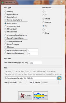
Since TraceWin version 2.4.2.0, the files “Desnity_PAR.dat” (for multiparticle) and “Density_Env.dat” (for envelope) replace the “Dist_Error_PAR.dat” and “Dist_Error_Env.dat” respectively. These new files contain much more data in order to visualize the transverse and longitudinal beam densities according to Z and some other beam parameters (all these data can come from the sum of statistical studies). All available charts are accessible via the Toolbox "Density". This tool is still able to read old density file version.
The following C++ example shows how density files are written.
These files replace also the obsolete file (particle loss distribution, “Dist_Error_Tot_PAR.loss”)
In case of statistical error study 2 new files are created name Density_tot_ENV.dat and Density_tot_PAR.dat witch contain the sum of all the simulation.
If the “Nbr of Step” parameter of the tab-sheet “Error” is bigger than 1 the name of the 2 files become for example for 5 steps
“Density_Tot_Env_0.2000.dat“ for 20%
“Density_Tot_Env_0.4000.dat“ for 40%,
…
“Density_Tot_Env_1.0000.dat“ for 100%,
Example to read the Density_XXX file.
#define den_year 2011
#define den_version 12
#include <stdio.h>
void Density_file_reading()
{
short int ver,year,vlong;
int nelp,Nrun,n=7,step;
float moy[n],moy2[n],maxb[n],minb[n],maxRb[n],minRb[n],rms_size[n],rms_size2[n],
rms_emit[3],rms_emit2[3],min_pos_moy[n],max_pos_moy[n],Zg,Xouv,Youv,dXouv,dYouv,
ib,Eouv,PhPouv,PhMouv,Mipowlost,Mapowlost,phaseF,phaseG;
LongInt Np=0,lost2,Milost,Malost,longfichier=0;
double powlost2;
// All the following tables have to be correctly initialized
LongInt *lost=NULL;
ULongInt **tab=NULL;
unsigned int **stab=NULL;
float **tabp=NULL,*powlost=NULL;
FILE *f=fopen64("Density_PAR.dat","rb");
if (f==NULL) {
printf("Error: Impossible to open Density file\n");
exit(1);
}
do {
/* The following sequence is repeated for each position (Zg) in the machine */
fread(&ver,sizeof(short int),1,f); /* Density file version : 3 to 12 */
fread(&year,sizeof(short int),1,f); /* year of development : 2011 */
fread(&vlong,sizeof(short int),1,f); /* vlong=1 if the number of particle is greater than 2e9 */
fread(&Nrun,sizeof(int),1,f); /* Number of run (1 for envelop or multiparticle simulation) more for statistical error studies */
fread(&nelp,sizeof(int),1,f); /* element # */
fread(&ib,sizeof(float),1,f); /* Beam courant (A) */
fread(&Zg,sizeof(float),1,f); /* Position (m), end of element or at step position calculation in field_map or in envelope mode */
fread(&Xouv,sizeof(float),1,f); /* Horizontal aperture */
fread(&Youv,sizeof(float),1,f); /* Vertical aperture */
if (ver>=9) {
fread(&dXouv,sizeof(float),1,f); /* Horizontal aperture shift */
fread(&dYouv,sizeof(float),1,f); /* Vertical aperture shift*/
}
fread(&step,sizeof(int),1,f); /* The beam is slice en step from max. to min. beam size */
/* n=7 (0:X(m)) (1:Y(m)) (2:Phase(°)) (3:Energy(MeV)) (4:R(m)) (5:Z(m)) (6:dp/p) */
fread(moy,sizeof(float),n,f); /* Beam average (m) for each plane */
fread(moy2,sizeof(float),n,f); /* Squared beam average (m2) for each plane (needed when Nrun>1) */
fread(maxb,sizeof(float),n,f); /* Maximum beam size (m) or particle excursion for each plane */
fread(minb,sizeof(float),n,f); /* Minimum beam size (m) or particle excursion for each plane */
if (ver>=11) {
fread(&phaseF,sizeof(float),1,f); /* Absolute beam phase*/
fread(&phaseG,sizeof(float),1,f); /* Absolute ref phase*/
}
if (ver>=10) {
fread(maxRb,sizeof(float),n,f); /* Minimum of Maximum beam size (m) or particle excursion for each plane (for range plot)*/
fread(minRb,sizeof(float),n,f); /* Maximum of Minimum beam size (m) or particle excursion for each plane (for range plot)*/
}
if (ver>=5) {
fread(rms_size,sizeof(float),n,f); /* rms beam size (m)*/
fread(rms_size2,sizeof(float),n,f); /* Quared beam rms size (m) */
}
if (ver>=6) {
fread(min_pos_moy,sizeof(float),n,f); /* Min. if the beam average (m) */
fread(max_pos_moy,sizeof(float),n,f); /* Maximum if the beam average (m) */
}
if (ver>=7) {
fread(rms_emit,sizeof(float),3,f); /* rms emi
ances, xx’, yy’, zdp (m.rad)*/
fread(rms_emit2,sizeof(float),3,f); /* Quared rms emittances, xx’, yy’, zdp (m.rad)2 */
}
if (ver>=8) {
fread(&Eouv,sizeof(float),1,f); /* Energy Acceptance (eV) */
fread(&PhPouv,sizeof(float),1,f); /* Positive Phase acceptance (deg)*/
fread(&PhMouv,sizeof(float),1,f); /* Negative Phase acceptance (deg)*/
}
fread(&Np,sizeof(LongInt),1,f);
if (Np>0) { //several linac simulation
/* particle lost and beam power lost for each linac */
if (lost!=NULL && powlost!=NULL) {
if (ver<12) {
for (int i=0;i<Nrun;i++) {
fread(&lost[i],sizeof(LongInt),1,f); /* Number of particle lost at position Zg */
fread(&powlost[i],sizeof(float),1,f); /* Beam power lost(W) at position Zg */
}
}
else {
for (int i=0;i<Nrun;i++) {
fread(&lost[i],sizeof(LongInt),1,f); /* Number of particle lost at position Zg */
}
if (ib>0) {
for (int i=0;i<Nrun;i++) {
fread(&powlost[i],sizeof(float),1,f); /* Beam power lost(W) at position Zg */
}
}
}
}
else fseeko64(f,Nrun*(sizeof(LongInt)+sizeof(float)),SEEK_CUR);
fread(&lost2,sizeof(LongInt),1,f); /* Squared particle number lost at position Zg */
fread(&Milost,sizeof(LongInt),1,f);/* Minimum particle lost at position Zg when Nrun>1 */
fread(&Malost,sizeof(LongInt),1,f);/* Maximum particle lost at position Zg when Nrun>1 */
fread(&powlost2,sizeof(double),1,f);/* Squared beam power lost(W) at position Zg */
fread(&Mipowlost,sizeof(float),1,f);/* Minimum beam power lost at position Zg when Nrun>1 */
fread(&Mapowlost,sizeof(float),1,f);/* Maximum beam power lost at position Zg when Nrun>1 */
/*tab or stab contains beam distribution from max. to min. size for each plane (7) slice in step*/
if (tab!=NULL && stab!=NULL) {
for (int j=0;j<n;j++) {
if (vlong==1) fread(tab[j],sizeof(ULongInt),step,f);
else fread(stab[j],sizeof(unsigned int),step,f);
}
}
else {
if (vlong==1) fseeko64(f,n*step*sizeof(ULongInt),SEEK_CUR);
else fseeko64(f,n*step*sizeof(unsigned int),SEEK_CUR);
}
if (ib>0) {
/* tabp contains beam power distribution from max. to min. size for X, Y and R planes */
if (tab!=NULL && stab!=NULL && tabp!=NULL) {
for (int j=0;j<3;j++) {
fread(tabp[j],sizeof(float),step,f);
}
}
else fseeko64(f,3*step*sizeof(float),SEEK_CUR);
}
}
/* next step */
/* break when Zg>=Linac length */
if (ftello64(f)+16>=longfichier) break;
} while (!feof(f));
fclose(f);
}
Dist_Error_Env.dat (OBSOLETE see Density_Env.dat file)
Contain the beam distribution at the end of each element after an envelope calculation. This file is created if “nbr of particles” is greater than 10 and “Use aperture element” of “Main” page is selected. During an error study the condition “nbr of particles” is sufficient. You can visualize these results in the “Error” page by setting the “Distribution file” and using the right buttons
Dist_Error_PAR.dat (OBSOLETE see Density_PAR.dat file)
Contain the beam distribution at the end of each element after a multiparticle calculation. This file is created either by PARTRAN or TOUTATIS. You can visualize these results in the “Error” page by setting the “Distribution file” and using the right buttons
§ N: Number of linac = 1
§ Element number
§ Element aperture (cm)
§ Element aperture (cm)
§
![]() (cm)
(cm)
§
![]() (cm2)
(cm2)
§
![]() (cm)
(cm)
§
![]() (cm2)
(cm2)
§
![]() (cm)
(cm)
§
![]() (cm2)
(cm2)
§ 100 integers corresponding to the particle distribution along the aperture divided in 100 steps.
§ 100 Doubles corresponding to the power distribution along the aperture divided in 100 steps.
§
![]()
§
![]()
§ Max particle lost
§ Min particle lost
§
![]() (w)
(w)
§
![]() (w)
(w)
§ Max power lost (w)
§ Min power lost (w)
In case of statistical error study 2 new files are created name Dist_Error_tot_ENV.dat and Dist_Error_tot_PAR.dat witch contain the sum of the 2 preceding files (N>1).
If the “Nbr of Step” parameter of the tab-sheet “Error” is bigger than 1 the name of the 2 files become for example for 5 steps
“Dist_Error_Tot_Env_0.2000.dat“ for 20%
“Dist_Error_Tot_Env_0.4000.dat“ for 40%,
…
“Dist_Error_Tot_Env_1.0000.dat“ for 100%,
The file “Steerer_Values.txt” is created after diagnostic position calculation. Its syntax is number of diagnostic follows by all the steerer strengths associated in T.m (Plane X and Y).
In case of statistical error study a new file named “Steerer_Values_Tot_X_XX.txt” is written including all the steerer strength of the whole linac simulated. A tool available in the “Errors” page-sheet allows to extract all useful statistical results from this file.
The file “Cav_set_point_res.txt” is created after envelope calculation. It contains the synchronous phase and Voltage for each RF cavity of the structure. Reference values and final tuned values are included.
In case of statistical error study a new file named “Cav_set_point_res_Tot_X_XX.txt” is written including all the cavity setting points of the whole linac simulated. A tool available in the “Errors” page-sheet allows to extract all useful statistical results from this file.
The file “Adjusted_Values.txt” is created after each diagnostic optimization adjusting some elements parameters.
In case of statistical error study a new file named “Adjusted_value_Tot_X_XX.txt” is written including all the element parameters adjusted of the whole linac simulated.
The file “MAGSTRIP1.LOS” is created only in multiparticle mode if option “Magnetic stripping” is selected in “Option” of multiparticle codes. You can directly exploit these results using “Stripping” button in tab-sheet “Graphs”. It contains the probability losses due to Lorentz magnetic stripping. The syntax is the following. (One line per element):
Number of element, Position (m), Energy (MeV), Losses probability
In case of statistical error study a new file named “MAGSTRIP1_TOT.LOS” is written including the probability sum of the whole linacs simulated. You can directly exploit these results using “Stripping losses probability results” button in “Errors” page. The syntax is the following (One line per element):
Number of element, Number of linac simulated, Sum of losses probability
The probability corresponding to Sum of Magnetic stripping probability divided by Number of linac simulated.
The file “GASSTRIP1.LOS” is created only in multiparticle mode if option “Gas stripping” is selected in “Option” of multiparticle codes and if command Gas pressure is included in the data file. It contains the probability losses due to Gas stripping. The syntax is the following. (One line per element):
Number of element, Position (m), Energy (MeV), Losses probability
In case of statistical error study a new file named “GASSTRIP1_TOT.LOS” is written including the probability sum of the whole linacs simulated. You can directly exploit these results using “Stripping losses probability results” button in “Errors” page. The syntax is the following (One line per element):
Number of element, Number of linac simulated, Sum of losses probability
The probability corresponding to Sum of Gas stripping probability divided by Number of linac simulated.
Losses_PAR.dat
Losses_PAR_TOT.dat (in statistical error study)
These ASCII files are created only while multiparticle simulation, if the option “Losses file“ is activated in the “Multparticle” page. These files contain all coordonates of each lost particles. The syntax of the file is described at the first line.
These following files are created while multiparticle simulation
part_dtl1.dst: Binary file containing the output beam distribution at the end of the linac.
part_rfq1.dst: Binary file containing the beam distribution at the entrance of the linac.
A .dst file use a binary format. It contains information of a beam at a given longitudinal position: number of particles, beam current, repetition frequency and rest mass as well as the 6D particles coordinates. The format is the following:
2xCHAR+INT(Np)+DOUBLE(Ib(mA))+DOUBLE(freq(MHz))+CHAR+
Np×[6×DOUBLE(x(cm),x'(rad),y(cm),y'(rad),phi(rad),Energie(MeV))]+
DOUBLE(mc2(MeV))
Comments:
§ CHAR is 1 byte long ,
§ INT is 4 bytes long,
§ DOUBLE is 8 bytes long.
§ Np is the number of particles,
§ Ib is the beam current,
§ freq is the bunch frequency,
§ mc2 is the particle rest mass.
dtl1.plt: Binary file containing the beam distribution at the end of each element (Ne). In the case of field map type elements, Nstep is greater than 1 (in fact, beam distributions are present at different positions along the length of the field map), for other elements Nstep is equal to 1. Note that the value of Nstep is not specified and that you have to read the data sequentially while monitoring Ne to know if you are leaving the field map.)
A .plt file use a binary format. It contains information of a beam at many longitudinal positions: longitudinal position, number of particles, beam current, repetition frequency and rest mass as well as the 6D particles (Np) coordinates. The format is the following according to compression level. The two first CHAR read define the compression level.
No compression (char1=125, char2=100):
2xCHAR+INT(Ne)+INT(Np)+DOUBLE(Ib(A))+DOUBLE(freq(MHz))+DOUBLE(mc2(MeV))+
Ne×[
Nstep×[
CHAR+INT(Nelp)+DOUBLE(Zgen)+DOUBLE(phase0(deg))+DOUBLE(wgen(MeV))+
Np×[
7×FLOAT(x(cm),x'(rad),y(cm),y'(rad),phi(rad),Energie(MeV),Loss)
]
]
]
Compression level 1 (char1=124, char2=99):
2xCHAR+INT(Ne)+INT(Np)+DOUBLE(Ib(A))+DOUBLE(freq(MHz))+DOUBLE(mc2(MeV))+
Ne×[
Nstep×[
CHAR+INT(Nelp)+DOUBLE(Zgen)+DOUBLE(phase0(deg))+DOUBLE(wgen(MeV))+
6×FLOAT(p0)
6×FLOAT(m0)
Np×[
7×SHORT_INT(x(cm),x'(rad),y(cm),y'(rad),phi(rad),Energie(MeV),Loss)
]
]
]
for (int i=0;i<=5;i++) {
k0[i]=(float)(m0[i] / 65534.);
}
for (int i=0;i<Np;i++) {
x[i] = k0[0]*((FLOAT)Np[0+i]+p0[0]);
x’[i] = k0[1]*((FLOAT)Np[1+i]+p0[1]);
y[i] = k0[2]*((FLOAT)Np[2+i]+p0[2]);
y’[i] = k0[3]*((FLOAT)Np[3+i]+p0[3]);
W[i] = k0[4]*((FLOAT)Np[4+i]+p0[4]);
P[i] = k0[5]*((FLOAT)Np[5+i]+p0[5]);
loss[i] =(FLOAT)Np[6+i];
}
Compression level 2 (char1=123, char2=98):
2xCHAR+INT(Ne)+INT(Np)+DOUBLE(Ib(A))+DOUBLE(freq(MHz))+DOUBLE(mc2(MeV))+
Ne×[
Nstep×[
CHAR+INT(Nelp)+DOUBLE(Zgen)+DOUBLE(phase0(deg))+DOUBLE(wgen(MeV))+
6×FLOAT(p0)
6×FLOAT(m0)
Np×[
8×UNSIGNED_CHAR(x(cm),x'(rad),y(cm),y'(rad),phi(rad),Energie(MeV),Loss)
]
]
]
for (int i=0;i<=5;i++) {
k0[i]=(float)(m0[i] / 255.);
}
for (int i=0;i<Np;i++) {
x[i] = k0[0]*((FLOAT)Np[0+i]+p0[0]);
x’[i] = k0[1]*((FLOAT)Np[1+i]+p0[1]);
y[i] = k0[2]*((FLOAT)Np[2+i]+p0[2]);
y’[i] = k0[3]*((FLOAT)Np[3+i]+p0[3]);
W[i] = k0[4]*((FLOAT)Np[4+i]+p0[4]);
P[i] = k0[5]*((FLOAT)Np[5+i]+p0[5]);
loss[i] =(FLOAT)Np[6+i]+256×(FLOAT)Np[7+i];
}
Compression level 3 (char1=122, char2=97):
Not relevant, don’t use this level of compression
Comments:
§ CHAR is 1 byte long,
§ UNSIGNED_CHAR is 1 byte long,
§ INT is 4 bytes long integer,
§ SHORT_INT is 8 bytes long integer.
§ FLOAT is 4 bytes long real.
§ DOUBLE is 8 bytes long real.
§ Ne is the number of different positions,
§ Np is the number of particles,
§ Ib is the beam current,
§ freq is the bunch frequency,
§ mc2 is the particle rest energy,
§ Nelp is the longitudinal element position,
§ Zgen is the longitudinal position in cm,
§ Phase0 & wgen are the phase and energy references of the beam,
At the end of a simulation, the list of the final errors applied on each element can be found on the calculation directory in the file “Error_Datas.txt”. A file using the same syntax can be use associated with the boith commands, ERROR_STAT_FILE & ERROR_DYN_FILE.
During a statistical error study, for each linac a file, “Error_Datas_XX.txt” is saved.
QUAD_ERROR dx(mm),dy(mm),drx(°),dry(°),drz(°),dG(%),L(mm),dG3(%),dG4(%),dG5(%),dG6(%)
CAV_ERROR dx(mm),dy(mm),drx(°),dry(°),drz(°),dE(%),dPhase(°),L(mm)
BEND ERROR dx(mm),dy(mm),drx(°),dry(°),drz(°),dg(%),dz(mm)
BEAM_ERROR dx(mm), dy(mm), dφ(°), dxp(mrad), dyp(mrad), de(MeV), dEx(%), dEy(%), dEz(%), mx(%), my(%), mz(%), dib(mA ),αxx’_min, αxx’_max, βxx’_min(mm/mrad), βxx’_max(mm/mrad), αyy’_min, αyy’_max, βyy’_min(mm/mrad), βyy’_max(mm/mrad), αzdp_min, αzdp_max, βzdp_min(mm/mrad), βzdp_max(mm/mrad)
ERROR_BEAM 0.0180812 0.029287 0 0.0815901 -0.0979198 -0 0 0 0 0 -0 0 -0 0 0 0 0 0 0 0 0 0 0 0 0
QUAD_ERROR [1] -0.0358043 -0.106052 -0.0152857 -0.0392236 0.0497174 -0.790136 0.73 0 -0 -0 0
QUAD_ERROR [2] -0.0629623 -0.053688 -0.0216135 -0.07538 0.0389759 0.0504835 0 0 -0 -0 0
CAV_ERROR [4] 0.00226118 0.00857076 0.00804547 0.000738873 0 0.785965 0.0847529 0.73
QUAD_ERROR [5] 0.0661981 -0.0781597 -0.0605019 0.0523095 0.0493564 0.0607798 0 0 0 0 0
CAV_ERROR [160] 0.00875094 0.00181656 -0.0293326 -0.0246627 0 0.618743 -0.408912 0.3
QUAD_ERROR [167] -0.0792799 -0.0387784 0.010346 0.00170561 0.193866 0.958619 0.13 0 0 -0 -0
QUAD_ERROR [168] -0.0792799 -0.0387784 0.010346 0.00170561 0.193866 0.958619 0.13 0 0 -0 -0
QUAD_ERROR [169] -0.0792799 -0.0387784 0.010346 0.00170561 0.193866 0.958619 0.13 0 0 -0 -0
QUAD_ERROR [170] -0.0792799 -0.0387784 0.010346 0.00170561 0.193866 0.958619 0.13 0 0 -0 -0
QUAD_ERROR [176] -0.0648002 0.0634561 -0.00654776 0.00490306 -0.162641 -0.214648 0.13 -0 0 0 0
CAV_ERROR [183] -0.000958443 -0.00685156 0.0171741 0.0266001 0 -0.0191761 0.132693 0.3
QUAD_ERROR [190] -0.0676107 0.0954914 -0.0285646 0.0129899 -0.0218936 0.436949 0.13 0 0 0 0
QUAD_ERROR [191] -0.0676107 0.0954914 -0.0285646 0.0129899 -0.0218936 0.436949 0.13 0 0 0 0
QUAD_ERROR [192] -0.0676107 0.0954914 -0.0285646 0.0129899 -0.0218936 0.436949 0.13 0 0 0 0
QUAD_ERROR [193] -0.0676107 0.0954914 -0.0285646 0.0129899 -0.0218936 0.436949 0.13 0 0 0 0
QUAD_ERROR [199] -0.0884702 0.103422 0.0626978 0.0526471 0.164511 -0.561579 0.13 0 0 0 0
CAV_ERROR [206] 0.00760207 0.00346884 0.00935432 -0.00380327 0 -0.965653 0.852592 0.3
[X] is the element number, L(mm) parameters can be use to find the particle coordinates at the input of the considered element.
Horizontal example:
![]() ,
, ![]()
The final results can be found on the calculation directory. Named “Error_study_Name_TRA.txt” when the result comes from an envelope calculation and “Error_study_Name_PAR.txt” when it is a PARTRAN study. The format of these files is the same for each kind of error. For each step of calculation one line of 32 parameters is written with the following format.
§ Step of error (0->1)
§ 1-(Nbr of particles)/(Nbr of particles, reference case)
§ (Emittance rms xx’,yy’,zz’)/ (Reference rms emittance xx’,yy’,zz’)-1
§ X beam center (m)
§ Y beam center (m)
§ X’ beam center (rad)
§ Y’ beam center (rad)
§ Energy beam center (keV)
§ Phase beam center (deg)
§ RMS Beam X size (m)
§ RMS Beam Y size (m)
§ RMS Beam X’ size (m)
§ RMS Beam Y’ size (m)
§ RMS Beam Energy size (keV)
§ RMS Beam Phase size (deg)
§ Halo parameter xx’
§ Halo parameter yy’
§ Halo parameter zz’
§ Horizontal dispersion (m)
§ Vertical dispersion (m)
§ Horizontal dispersion / dz
§ Vertical dispersion /dz
§ Apha_XX’
§ Beta_XX’ (m/rad)
§ Apha_YY’
§ Beta_YY’ (m/rad)
§ Apha_PE
§ Beta_PE (deg/MeV)
§ Emittance 4D/Reference emittance 4D-1
§ Emittance 6D/Reference emittance 6D-1
All these values are relative to the output beam without errors.
In case of statistical study, where each step of calculation contains several runs, the format becomes:
§ Step of error (0->1)
§ AVERAGE(1-(Nbr of particles)/(Nbr of particles, reference case))
§ (AVERAGE(Emittance rms xx’,yy’,zz’))/ (Reference rms emittance xx’,yy’,zz’)-1
§ RMS(X beam center (m))
§ RMS(Y beam center (m))
§ RMS(X’ beam center (rad))
§ RMS(Y’ beam center (rad))
§ RMS(Energy beam center (keV))
§ RMS(Phase beam center (deg))
§ AVERAGE(RMS Beam X size (m))
§ AVERAGE(RMS Beam Y size (m))
§ AVERAGE(RMS Beam X’ size (m))
§ AVERAGE(RMS Beam Y’ size (m))
§ AVERAGE(RMS Beam Energy size (keV))
§ AVERAGE(RMS Beam Phase size (deg))
§ AVERAGE(Halo parameter xx’)
§ AVERAGE(Halo parameter yy’)
§ AVERAGE(Halo parameter zz’)
§ AVERAGE(Apha_XX’)
§ AVERAGE(Beta_XX’ (m/rad))
§ AVERAGE(Apha_YY’)
§ AVERAGE(Beta_YY’ (m/rad))
§ AVERAGE(Apha_PE)
§ AVERAGE(Beta_PE (deg/MeV))
§ AVERAGE(X beam center (m))
§ AVERAGE(Y beam center (m))
§ AVERAGE(X’ beam center (rad))
§ AVERAGE(Y’ beam center (rad))
§ AVERAGE(Energy beam center (keV))
§ AVERAGE(Phase beam center (deg))
And a file call “Error_study_Name_TRA_tot.txt” or “Error_study_Name_PAR_tot.txt” is written containing all run results.
The final multiparticle results contain one line by element output, the first line being the input beam parameters. The format is like following.
§ Element number
§ Element position (m)
§ Relativistic parameters: (γ-1)
§ Centroid position: x(mm), y(mm), j(deg), x’(mrad), y’(mrad), W(MeV)
§ RMS_SIZE [ σx(mm), σy(mm), σj(deg) ]
§ áxx'ñ (mm.mrad), áyy'ñ (mm.mrad), áWφñ (deg.MeV)
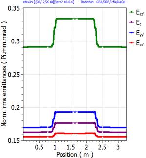
§ Normalized rms emit: xx’(π.mm.mrad), yy’(π.mm.mrad), jW (π.deg.MeV).(*)
§ Halo parameters: (Hxx’, HYY’, Hz.dp/p)
§ Number of particles
§ Phase advance with space charge (deg/mm): σx, σy, σz.
§ Emittance at 99%: εxx’, εyy’, εz.dp/p
§ Djs (°), average beam phase - reference beam phase
§ DWs (MeV), average beam energy - reference beam energy
§ Beam currant (mA) used for space charge calculation
§ Aperture (mm)
§ Normalized 4D transverse emittance Exx’yy’ (π.mm.mrad)2
§ Normalized rms emit (π.mm.mrad): εrr’
§ Phase advance with space charge (deg/mm): σr
§ Lost power (W)
§ Maximum excursion particle : Xmax(mm), Ymax(mm),
§ Normalized long. rms emit: εz.dp/p (π.mm.mrad)(*) [replace jW(deg.MeV) value]
§ RMS_SIZE [σz(mm)]
§ áz.dp/pñ (mm.mrad)(*)(**)
§ Dispersion: Dh (mm), Dv(mm)
§ Derivative dispersion: Dh’ (mrad), Dv’(mrad)
§ σxy
§ σx’y’
§ σxy’
§ σx’y
![]() with
with ![]() , same equations
for phase spaces [yy'] and [z. dp/p] to get σy and σdp/p
, same equations
for phase spaces [yy'] and [z. dp/p] to get σy and σdp/p
(*) Since TraceWin version 2.1.0.0 longitudinal rms emittance jW is set to zero and has been replaced by εz.dp/p
(**) εz.dp/p is expressed in π.mm.mrad not in π.mm.% like in GUI output display. The conversion is 1.π.mm.mrad = 10. π.mm.%
User has the possibility to set the random seed, in “main” page, in order to regenerate an error case. For remote computing the seed values are saved in a file name “Random_seed.log”.
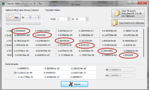
“Transfer_matrix1.dat” file contains the 6x6 tranfer matrix of the structure from the first to the last element. The syntax is similar to the outputs visible in the tool “Structure tranfer Matrix” from the “Charts” tab-sheet.
In “Charts” tab-sheet the option “Include structure errors in transfer matrix” defined if the transfer matrix shown in the corresponding tools or saved into the file take or not into account the errors applied to the structure.
During error study, if option “Keep all result files” is selected in tab_shhet “Errors” a list of file ““Transfer_matrix1.dat_XXX” is created.
Circular or rectangular aperture
Electromagnetic static or RF field (Field Map)
Field map with curved reference trajectory
|
Mnemonic |
Parameter |
Definition |
|
DRIFT |
L |
Length (mm) |
|
R |
Aperture (mm) |
|
|
|
Ry |
Aperture (mm) |
|
|
Rx_shift |
Orizontal aperture shift (mm) |
|
Ry_shift |
Vertical aperture shift (mm) |
If Ry equals 0, aperture is circular with R radius.
If Ry is not equal 0, aperture is rectangular with R the half dimension in x plane and Ry in y plane.
Rx/y_shift allows to introduce a non-cental aperture.
Link to Drift matrix
|
Mnemonic |
Parameter |
Definition |
|
QUAD |
L |
Length (mm) |
|
QUAD_SPEC |
G |
Magnetic field gradient (T/m) |
|
R |
Aperture (mm) |
|
|
Θ |
Skew Angle (°) |
|
|
G3 / u3 |
Sextupole gradient (T/m2) or relative sex. component |
|
|
G4 / u4 |
Octupole gradient (T/m3) or relative oct. component |
|
|
G5 / u5 |
Decapole gradient (T/m4) or relative deca. component |
|
|
|
G6 / u6 |
Dodecapole gradient (T/m5) or relative dode. component |
|
GFR |
Good field radius (mm) |
Attention to the TraceWin gradient definition.
Red values are optional.
If L equals 0, the quadrupole is simulated as thin lens and all gradients have to be replaced by their integral (over longitudinal direction) values.
Multipole kicks are applied at the middle of the quadrupole.
If GFR is non null, un are relative multipole components will defined such as:
![]()
QUAD_SPEC : is similar to an usual QUAD element except that it is focusing in both horizontal and vertical plane.
Link to Quadrupole matrix
|
Mnemonic |
Parameter |
Definition |
|
CONF |
L |
Length (mm) |
|
ns |
Number of spce-charge kick (Partran only) |
|
|
R |
Aperture (mm) |
|
|
kx |
Horizontal focusing |
|
|
ky |
Vertical focusing |
|
|
kz |
Longitudinal focusing |
Link to Containment channel
Beam Rotation
|
Mnemonic |
Parameter |
Definition |
|
BEAM_ROT |
θxy |
Angle (°) in the XY space around Z |
|
θxz |
Angle (°) in the XZ space around Y |
|
|
θyz |
Angle (°) in the YZ space around X |
|
|
dx |
X shift (mm) |
|
|
dy |
Y shift (mm) |
|
|
dxp |
Xp shift (mrad) |
|
|
dyp dz centroid_flag |
Yp shift (mrad) Z (mm) 0 : turn around gravity center |
Rotations are first performed in the following order: around Z, Y and X, and finally the shifts. Centroid_flag defines if the rotation is done around beam center of gravity (=0) or if the rotation is done around the synchronous particle (also applied on beam centroid, except energy). BEAM_ROT is considered as an element
Link to Beam rotation matrix
Thin Lens
|
Mnemonic |
Parameter |
Definition |
|
THIN_LENS |
fx |
Focal Length (m) |
|
fy |
Focal Length (m) |
|
|
R |
Aperture (mm) |
Link to Thin lens matrix
|
Mnemonic |
Parameter |
Definition |
|
THIN_MATRIX |
lg |
Length (mm) |
|
|
a00 to a55 |
Matrix terms, row per row |
The 36 terms of a transfer matrix have to be set row by row from a00 to a55. Length, lg, is just used in graphic view.
Link to matrix format R
The associated phase-space are respectively: x (m), x’ (rad), y (m), y’ (rad), z (m), dp/p (rad)
Quadrupole Example: THIN_MATRIX 10.0 1 0 0 0 0 0 -2.5 1 0 0 0 0 0 0 1. 0 0 0 0 0 2.5 1 0 0 0 0 0 0 1 0 0 0 0 0 0 1
|
Mnemonic |
Parameter |
Definition |
|
QUAD_ELE |
L |
Length (mm) |
|
Vo |
Voltage between electrodes (V) |
|
|
R |
Aperture (mm) |
|
|
Θ |
Skew Angle (°) |
|
|
V3 / u3 |
Sextupole voltage gradient component (V/m) or relative |
|
|
V4/ u4 |
Octupole voltage gradient component (V/m2) or relative |
|
|
V5/ u5 |
Decapole voltage gradient component (V/m3) or relative |
|
|
|
V6/ u6 |
Dodecapole voltage gradient component (V/m4) or relative |
|
GVR |
Good voltage radius (mm) |
Attention to the TraceWin gradient definition.
Vo is the voltage difference between neighboring electrodes (+Vo/2 on one and –Vo/2 on its neighbors). The distance between opposite electrodes is 2R.
In order to keep coherence with old TraceWin version, all electrostatic components are in voltage: (V) and not in field: E (V/m)
If L equals 0, electrostatic quadrupoles are simulated as thin lens and all voltage components have to be replaced by their integral (over longitudinal direction) values.
Multipole kicks are applied at the middle of the electrostatic quadrupole.
If VFR is non null, un are relative multipole components will defined such as:
![]()
Link to Quadrupole matrix
|
Mnemonic |
Parameter |
Definition |
|
GAP |
E0TL |
Effective gap voltage (V) |
|
θs |
RF phase (deg) (absolute or relative) |
|
|
R |
Aperture (mm) |
|
|
P |
0: θs is relative, 1: θs is absolute phase, 2: θs is relative + beam phase error set to 0 3: θs if set to 0 all phases are absolute including phase error resulting in preceding structures. If not set to 0, θs is the relative phase including phase error resulting in preceding structure. |
|
|
βs |
Particle reduced velocity |
|
|
Ts |
Transit time factor |
|
|
kT’s |
(*) |
|
|
k²T”s |
(*) |
Red parameters are optional
(*) See Transit time factor definition
Bunched cavity or thin gap matrix
|
Mnemonic |
Parameter |
Definition |
|
CAVSIN |
L |
Length (mm) |
|
N |
Cell number |
|
|
EoT |
Average accelerating field (V/m) |
|
|
θs |
Phase of the synchronous particle at the entrance(deg)(*) |
|
|
R |
Aperture (mm) |
|
|
P |
1: θs is absolute phase, 0: θs is relative |
(*) Use SET_SYNC_PHASE command in order to change this phase as the synchronous phase
Link to Sinus cavity or CCL matrix
|
Mnemonic |
Parameter |
Definition |
|
BEND |
α |
Bend angle in the rotation plane (deg) |
|
|ρ| |
Curvature radius of central trajectory (mm) |
|
|
N |
Field gradient index |
|
|
R |
Aperture (mm) |
|
|
HV |
0 : horizontal, 1 : vertical |
Warning: A bend always have to be surrounded by an edge element, even if edge is set to zero.
By definition: a positive bend (denoted α>0) bends the trajectory to the right in the horizontal plane, whatever the sign of the particle charge state.
The field gradient index is treated in the first order and applies only for horizontal bending.
Link to Bending magnet matrix
|
Mnemonic |
Parameter |
Definition |
|
EDGE |
b |
Pole face rotation angle (deg) |
|
|ρ| |
Curvature radius of bend (mm) |
|
|
G |
Total gap of magnet (mm) |
|
|
K1 |
Fringe-field factor (default = 0.45) |
|
|
K2 |
Fringe-field factor (default = 2.80) |
|
|
R |
Aperture (mm) |
|
|
HV |
0 : horizontal, 1 : vertical |
By definition: an edge focalizes if β < 0, whatever the curvature radius sign, the bending angle sign and the particle charge state.
Set K1 and K2 to a very small values to disable fringe field estimation.
G is used for particle loss estimation in bend.
Link to Edge angle on bending magnet matrix
|
Mnemonic |
Parameter |
Definition |
|
BEND_ELE |
α |
Bend angle in the rotation plane (deg) |
|
|ρ| |
Curvature radius of central trajectory (mm) |
|
|
ne |
1:Cylindrical, 2:Spherical, 3:Toroidal |
|
|
R |
Aperture (mm) |
|
|
HV |
0 : horizontal, 1 : vertical |
By definition: a positive bend (denoted α>0) bends the trajectory to the right in the horizontal plane, whatever the sign of the particle charge state.
Only cylindrical bends are available in multiparticle mode.
|
Mnemonic |
Parameter |
Definition |
|
APERTURE |
dx |
X (mm) half width or radius hole (pepperpot) |
|
dy |
Y (mm) half width or distance between hole (pepperpot) |
|
|
n |
Type : 0 : Rectangular aperture 1 : Circular aperture 2 : Pepperpot mode 3 : Rectangular aperture with dx & dy corresponding to a beam fraction intercepted by the aperture (adjusted with 0.1 mm step) if value <1, otherwise dx or dy are used as type=0 4 : Horizontal finger with dx=finger center position, dy=total finger width. 5 : vertical finger with dx=finger center position, dy=total finger width. 6 : Ring aperture if particle radius, r>dy or r<dx with (dx<dy) particle is lost. |
|
Mnemonic |
Parameter |
Definition |
|
SPACE_CHARGE_COMP |
k |
Beam current is compensated by a factor k |
Set a beam new current: Ib = (1-k)×Ib.
|
Mnemonic |
Parameter |
Definition |
|
CURRENT |
Ib |
Beam current (mA) |
Set a beam new current: Ib (mA).
|
Mnemonic |
Parameter |
Definition |
|
SOLENOID |
L |
Length (mm) |
|
B |
Magnetic field (T) |
|
|
R |
Aperture (mm) |
Solenoid treated as thick length.
Link to Solenoid matrix
|
Mnemonic |
Parameter |
Definition |
|
THIN_STEERING |
BLx or ELx |
x-component (T.m or V) |
|
Bly or ELy |
y-component (T.m or V) |
|
|
r |
Aperture (mm) |
|
|
Elec |
0: magnetic deviation (default) 1: electric deviation |
Transverse kick.
Link to Thin steering matrix
|
Mnemonic |
Parameter |
Definition |
|
DTL_CEL |
L |
Cell length (mm) |
|
Lq1 |
First ½ quadruploe length (mm) |
|
|
Lq2 |
Second ½ quadruploe length (mm) |
|
|
gc (*) |
Gap center shift (mm) (*) |
|
|
B1’ |
First magnetic field gradient (T/m) |
|
|
B2’ |
Second magnetic field gradient (T/m) |
|
|
EoTL |
Effective gap voltage (V) |
|
|
θs |
RF phase (deg) |
|
|
R |
Aperture (mm) |
|
|
P (**) |
0: θs is relative (**), 1: θs is absolute phase, 2: θs is relative + beam phase error set to 0 3: θs if set to 0 all phases are absolute including phase error resulting in preceding structures. If not set to 0, θs is the relative phase including phase error resulting in preceding structure. |
|
|
βs |
Particle reduced velocity |
|
|
Ts |
Transit time factor |
|
|
kT’s |
(***) |
|
|
k²T”s |
(***) |
Define a cell of a classical Drift Tube Linac (DTL).
(*) The gc(mm) dimension
is defined as: gap position ![]()
(**) This following example is the most realistic RF sequence: All synchronous phase are absolute phase and calculated according to the cell lengths, excepted for the first one which is set to the relative value. The phase error resulting in preceding structures is taken into account. You can canceled the preceding structure phase error by replacing type 3 by type 2 for the first cell
LATTICE 4 1
DTL_CEL 68.729 22.5 22.5 0.0125565 52.5 -52.5 176568 -30 10 3 0.0807374 0.778491 -0.377246 -0.1456
DTL_CEL 70.4468 22.5 22.5 0.00912044 -52.5 -52.5 182799 0 10 3 0.0827489 0.786305 -0.366349 -0.150419
DTL_CEL 72.1883 22.5 22.5 0.00491998 -52.5 52.5 188980 0 10 3 0.0847886 0.79329 -0.356535 -0.154494
DTL_CEL 73.9529 22.5 22.5 0.000837313 52.5 49.5 195297 0 10 3 0.0868553 0.800245 -0.346592 -0.157865
DTL_CEL 75.74 22.5 22.5 -0.0035088 49.5 -49.5 201675 0 10 3 0.0889485 0.806881 -0.336968 -0.16056
(**) See Transit time factor definition
Red parameters are optional.
If βs does not equal 0, Ts is mandatory.
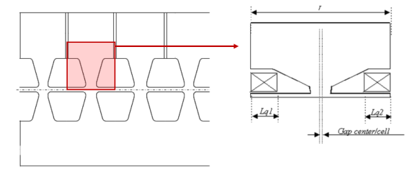
Link to DTL cell matrix
|
Mnemonic |
Parameter |
Definition |
|
NCELLS |
Mode |
(0)2π, (1)π, (2)π & 2π |
|
Nc |
Number of cell |
|
|
βg |
Geometric β > 0: all cell lengths are the same according to βg = 0: cell lengths are set according to beam velocity < 0: cell lengths are set according to an initial beam velocity –βg, which is increasing from cell to cell according to θs and EoT parameters. |
|
|
EoT |
Effective gap voltage (V/m) |
|
|
θs |
RF phase at the first gap position (deg) (**) |
|
|
R |
Aperture (mm) |
|
|
P |
0: θs is relative , 1: θs is absolute phase, 2: θs is relative + beam phase set to 0 |
|
|
kEoTi |
Input field correction, Eo = Eo*(1+k) |
|
|
kEoTo |
Output field correction, Eo = Eo*(1+k) |
|
|
dzi |
First gap displacement (mm) |
|
|
dzo |
Last gap displacement (mm) |
|
|
βs |
Particle reduced velocity |
|
|
Ts |
Transit time factor of the middle gaps |
|
|
kT’s |
(*) |
|
|
k²T”s |
(*) |
|
|
Ti |
Transit time factor of the input gaps |
|
|
kT’i |
(*) |
|
|
k²T”i |
(*) |
|
|
To |
Transit time factor of the output gaps |
|
|
kT’o |
(*) |
|
|
k²T”o |
(*) |
Modelisation of a multicell cavity by a set of gaps, with one gap at the middle of each cell.
Red parameters are optional
If βs is not equal to 0 Ts become needed
(*) See Transit time factor definition
(**) Use SET_SYNC_PHASE command in order to change this phase as the synchronous phase
Link to Cavity multi-gap matrix
|
Mnemonic |
Parameter |
Definition |
|
RFQ_CELL |
V |
Effective gap voltage (V) |
|
Ro |
Vane average radius (mm) (*) |
|
|
A10 |
Acceleration parameter |
|
|
m |
Vane modulation |
|
|
L |
Cell length (mm) |
|
|
θs |
RF phase (deg) |
|
|
Type |
|
|
|
Tc |
Transverse curvature (mm) |
|
|
- |
Not used any more |
|
|
|
a |
Minimum radius (**) |
(*) Vane geometry plotted in envelope chart is made for illustrate the RFQ_CELL element. It’s a rought drawing, expecialy for front-end cells.
(**) Optional parameter, but necessary defined for TWOTERM RFQ.
Link to RFQ cell matrix
Diagnostics measure beam properties at given position.
These measurements are used for the automatic tuning of transport elements to set the measured beam properties to wanted ones. The diagnostics and the associated adjustable transport elements are then linked with a common number. The association is made by preceding the transport elements with the adjust commands followed by the number of the associated diagnostics. The tuning is made in the order of the diagnostic numbers.
In these conditions, a uniform random measurement error is used according to the diagnostic accuracy. If accuracy > 0, the errors are uniformly distributed between ± accuracy value. If accuracy < 0, the errors are Gaussian distributed; accuracy value is then the rms value of the distribution.
|
Mesured property |
Mnemonic |
Parameter |
Definition |
|
DIAG_CURRENT |
N |
Diagnostic number |
|
|
|
Ib |
Wanted beam current (mA) or transmission (%) [both could be 0] If input beam current is 0 or flag parameter is not 0 transmission will be used. |
|
|
|
|
dIb |
Accuracy (mA) or (%) |
|
|
|
flag |
|
|
|
|
|
|
|
Delta Current |
DIAG_DCURRENT |
N |
Diagnostic number |
|
(2 are needed) |
|
Ibn-Ibn-1 |
Wanted Δcurrent (mA) or Δtransmission (%) [both could be 0] If input beam current is 0 or flag parameter is not 0, transmission will be used. |
|
|
|
dIb |
Accuracy (mA) or (%) |
|
|
|
flag |
|
|
|
|
|
|
|
DIAG_POSITION |
N |
Diagnostic number |
|
|
|
|
X |
Wanted X beam position (mm), (If X<1e50) |
|
|
|
Y |
Wanted Y beam position (mm), (If Y<1e50) |
|
|
|
dm |
Diagnostic Accuracy (mm) |
|
|
|
|
|
|
Delta position |
DIAG_DPOSITION |
N |
Diagnostic number |
|
|
|
X-Y |
Wanted X-Y beam position (mm) |
|
|
|
dm |
Diagnostic Accuracy (mm) |
|
|
|
|
|
|
Divergences |
DIAG_DIVERGENCE |
N |
|
|
|
|
X’ |
Wanted X divergence (mrad), (If Y’<1e50) |
|
|
|
Y’ |
Wanted Y divergence (mrad), (If Y’<1e50) |
|
|
|
dm |
Diagnostic Accuracy (mrad) |
|
|
|
|
|
|
Delta Divergence |
DIAG_DDIVERGENCE |
N |
Diagnostic number |
|
|
|
X’-Y’ |
Wanted X-Y divergence (mrad) |
|
|
|
dm |
Diagnostic Accuracy (mrad) |
|
|
|
|
|
|
Full Width at Half |
DIAG_SIZE_FWHM |
N |
Diagnostic number |
|
Maximum (FWHM) |
|
Sx |
Wanted FHHM X size (mm) (If ≠ 0) |
|
|
|
Sy |
Wanted FHHM Y size (mm) (If ≠ 0) |
|
|
|
ΔP |
Wanted FHHM Phase spread (°) (If ≠ 0) |
|
|
|
Dm |
Size Accuracy (mm) |
|
|
|
dΔP |
Phase spread Accuracy (°) |
|
|
|
fo |
ΔP Low-pass filter frequency (MHz) |
|
|
|
|
|
|
DIAG_SIZE |
N |
Diagnostic number |
|
|
|
|
Sx |
Wanted X rms size (mm) (If ≠ 0) |
|
|
|
Sy |
Wanted Y rms size (mm) (If ≠ 0) |
|
|
|
ΔP |
Wanted rms Phase spread (°) (If ≠ 0) |
|
|
|
Dm |
Size Accuracy (mm) |
|
|
|
dΔP |
Phase spread Accuracy (°) |
|
|
|
fo |
ΔP Low-pass filter frequency (MHz) |
|
|
|
|
|
|
Divergences |
DIAG_SIZEP |
N |
Diagnostic number |
|
|
Sx’ |
Wanted X’rms divergence (mrad) (If ≠ 0) |
|
|
|
|
Sy’ |
Wanted Y’rms divergence (mrad) (If ≠ 0) |
|
if S<0 Twiss |
|
ΔW |
Wanted rms Energy spread (MeV) (If ≠ 0) |
|
parameter alpha will |
|
Dm |
Divergence Accuracy (mrad) |
|
set <0 |
|
dW |
Energy spread Accuracy (%) |
|
|
|
|
|
|
Delta Full Width at |
DIAG_DSIZE_FWHM |
N |
Diagnostic number |
|
Half Maximum |
|
xn-yn |
Wanted x-y FWHM delta size (mm) |
|
(FWHM) |
|
dm |
dx-y size Accuracy (mm) |
|
|
|
|
|
|
Delta size |
DIAG_DSIZE |
N |
Diagnostic number |
|
Xrms-Yrms |
|
xn-yn |
Wanted x-y rms beam delta size (mm) |
|
|
|
dm |
dx-y size Accuracy (mm) |
|
|
|
|
|
|
Delta Full Width at |
DIAG_DSIZE2_FWHM |
N |
Diagnostic number |
|
Half Maximum |
|
xn-xn-1 |
Wanted x HWHM delta size (mm) |
|
between 2 positions |
|
yn-yn-1 |
Wanted y HWHM delta size (mm) |
|
(At least 2 are |
|
dm |
dx & dy size accuracy (mm) |
|
needed) |
|
|
|
|
Delta size |
DIAG_DSIZE2 |
N |
Diagnostic number |
|
between 2 positions |
|
xn-xn-1 |
Wanted x rms beam delta size (mm) |
|
(At least 2 are |
|
yn-yn-1 |
Wanted y rms beam delta size (mm) |
|
needed) |
|
dm |
dx & dy size accuracy (mm) |
|
|
|
|
|
|
Delta phase spread |
DIAG_DSIZE3 |
N |
Diagnostic number |
|
Measurement 2 |
|
ΔPn-ΔPn-1 |
Wanted rms delta phase spread (°) |
|
(At least 2 are |
|
dΔP |
Phase spread accuracy (°) |
|
Needed) |
|
fo |
dΔP Low-pass filter frequency (MHz) |
|
|
|
|
|
|
Delta divergence |
DIAG_DPSIZE2 |
N |
Diagnostic number |
|
between 2 positions |
|
x'n-x’n-1 |
Wanted x’ rms beam delta div. (mrad) |
|
(At least 2 are |
|
y’n-y’n-1 |
Wanted y’ rms beam delta div. (mrad) |
|
needed) |
|
dpm |
dx' & dy’ div. accuracy (mrad) |
|
|
|
|
|
|
DIAG_PHASE |
N |
Diagnostic number |
|
|
|
|
Θ |
Wanted centroïd Phase (°) |
|
|
|
|
|
|
Energy measurement |
DIAG_ENERGY |
N |
Diagnostic number |
|
|
|
W |
Wanted Energy (MeV) |
|
|
|
dw |
Accuracy (%) |
|
|
|
|
|
|
Beam energy - Perfect |
DIAG_DENERGY |
N |
Diagnostic number |
|
linac energy measurement |
|
W |
Wanted Delta Energy (MeV) |
|
|
|
dw |
Accuracy (%) |
|
|
|
|
|
|
Energy gain |
DIAG_W_GAIN |
N |
Diagnostic number |
|
between 2 positions |
|
Wn-Wn-1 |
Wanted erngy gian (MeV) |
|
(At least 2 are |
|
dw |
Accuracy (%) |
|
needed) |
|
(Parameters set to the second diagnostics) |
|
|
Luminosity |
DIAG_LUMINOSITY |
N |
Diagnostic number |
|
|
|
Lu |
Wanted luminosity (mm-²) |
|
|
|
Dlu |
Luminosity accuracy (mm-²) |
|
|
|
|
|
|
Waist setting |
DIAG_WAIST |
N |
Diagnostic number |
|
|
|
fx |
XX’ waist asked (for fx not equal to 0) |
|
|
|
fy |
YY’ waist asked (for fy not equal to 0) |
|
|
|
dxy |
Transverse waist Accuracy |
|
|
|
|
|
|
Achromat setting |
DIAG_ACHROMAT |
N |
Diagnostic number |
|
|
|
Ele# (**) |
First element number (**) |
|
|
|
f1 |
If =1 set achromatic position |
|
|
|
f2 |
If =1 set achromatic angle |
|
|
|
plan |
0 : X or Y or both planes acccoding to bend direction are concerned 1 : only X plan is concerned 2 : only Y plan is concerned 3 : both planes are concerned
|
|
Emittance setting |
DIAG_EMIT |
N |
Diagnostic number |
|
(rms values) |
|
Exx’ |
Wanted emittance if greater than 0 |
|
|
|
Eyy’ |
Wanted emittance if greater than 0 |
|
|
|
Epw |
Wanted emittance if greater than 0 |
|
|
|
|
|
|
Emittance setting |
DIAG_EMIT_99 (*) |
N |
Diagnostic number |
|
(99% value or others) |
|
Exx’ |
Wanted emittance if greater than 0 |
|
|
|
Eyy’ |
Wanted emittance if greater than 0 |
|
|
|
Epw |
Wanted emittance if greater than 0 |
|
|
|
|
|
|
Halo setting |
DIAG_HALO |
N |
Diagnostic number |
|
|
|
Hx |
Wanted haloX if greater than 0 |
|
|
|
Hy |
Wanted haloY if greater than 0 |
|
|
|
Hz |
Wanted haloZ if greater than 0 |
|
|
|
|
|
|
Transfer matrix |
DIAG_SET_MATRIX |
N |
Diagnostic number |
|
setting |
|
Ele# (**) |
Transfer matrix form element number, Ele#, to diag. position (**) |
|
|
|
Row(i) |
Row transfer matrix term |
|
|
|
Column(j) |
Column transfer matrix term |
|
|
|
k |
Corrector coefficient |
|
|
|
Mij |
Wanted transfer matrix term value |
|
Beam Twiss parameters setting
Parameter is used if it is not equal to 0,
If you want α=0 set very small α |
DIAG_TWISS |
N |
Diagnostic number |
|
αxx' |
Wanted alpXX’ |
||
|
|
βxx’ |
Wanted betXX’ (mm/mrad) |
|
|
|
αyy' |
Wanted alpYY’ |
|
|
βyy’ |
Wanted betYY’ (mm/mrad) |
||
|
αzdp/p |
Wanted alpZdp/p |
||
|
βzdp/p |
Wanted betZdp/p (mm/mrad) = 10 x time betZdp/p (mm/%) |
||
|
Make equal 2 beam Twiss parameters between 2 positions or more, (At least 2 are needed). The flag parameters must be defined in the first diagnostics to decide which quantity will be equalised.
|
DIAG_DTWISS |
N |
Diagnostic number |
|
fαxx' |
(1/0) |
||
|
fβxx’ |
(1/0) |
||
|
fαyy' |
(1/0) |
||
|
fβyy’ |
(1/0) |
||
|
fαzdp/p |
(1/0) |
||
|
fβzdp/p |
(1/0)
|
||
|
Make equal transverse Twiss parameter at diagnostic position |
DIAG_DTWISS2 |
N |
Diagnostic number |
|
|
fα |
If (fα=1) αxx’ – αyy’ is set to 0 |
|
|
|
fβ |
If (fβ=1) βxx’ – βyy’ is set to 0
|
|
|
Beam separation setting |
DIAG_SEPARATION |
N k |
Diagnostic number Correction factor (set 1) |
|
|
S |
Wanted separation (ks.Size/Position+kc.Position) |
|
|
|
|
0/1 |
0 for X plane, 1 for Y |
|
|
ks |
Weigth on separation |
|
|
|
kc |
Weigth on position |
|
|
|
|
|
|
|
Limit beam size max |
DIAG_SIZE_MAX (***) |
N N_ele
Sx0 |
Diagnostic number Number of upstream elements concerned Wanted max beam size X (mm), if !=0 |
|
Limit beam size min |
DIAG_SIZE_MIN (***) |
Sy0 |
Wanted max beam size Y (mm), if !=0 |
|
|
Sz0 |
Wanted max beam size Z (mm,deg), if !=0 If Sz < 0 Z size in mm otherwise in deg |
|
|
|
Flag_cent |
If 1, beam size includes beam centroid |
|
|
|
|
|
|
|
Set beam phase advance |
DIAG_PHASE_ADV |
N Ele# (**)
σx0 |
Diagnostic number Phase advance form element number, Ele#, to diag. position (**) Wanted X phase advance (deg), if !=0 |
|
|
σy0 σz0 |
Wanted Y phase advance (deg), if !=0 Wanted Z phase advance (deg), if !=0
|
|
|
Set beam beta |
DIAG_BETA |
N |
Diagnostic number |
|
|
|
βx |
Wanted betX (mm/mrad) if >0 |
|
|
|
βy |
Wanted betY (mm/mrad) if >0 |
|
|
|
βz |
Wanted betZ (mm/(dp/p)) if >0 |
|
|
|
f |
0: Twiss beta / 1: Beta function |
|
|
|
Dm |
Accuracy
|
|
Set delta Beam beta |
DIAG_DBETA |
N |
Diagnostic number |
|
|
|
βx - βy |
Wanted Delta beta (mm/mrad) |
|
|
|
f |
0: Twiss beta / 1: Beta function |
|
|
|
Dm |
Accuracy |
(*) 99% fraction must be set in “Multiparticle” tabsheet, then go to “99.XX% emittance and halo”,then select the fraction you want.
(**) if ( Ele#>0 ) then Ele# is absolute
if ( Ele#<0 ) then Ele# is relative, e.g. -15 means relative to location 15 elements upstream.
TraceWin can be used to verify if a beam line contains enough diagnostics to control the beam and correct the errors coming from the input beam or from the different element errors. In order to put one diagnostics in the line use the elements “DIAG_…” followed by the diagnostic number and the wanted parameters which have to be imposed at the diagnostic location (current, position, size or emittance). Precede the associated adjustable transport elements by the adjust commands followed by the number of the associated diagnostic.
There are two ways of using these diagnostics. The first one is for example to see if your design is able to control the beam position at a given location when you input beam is not at the center or if a few elements, like steerers induce misalignment. The second way is to use diagnostics in an error study in order to see if you scheme of misalignment correction for example is efficient enough.
The diagnostics adjustments are independent process, which occurs after the matching process. If any diagnostic element is present any adjustment is started. Finally, at the end of a line design process, only diagnostic elements should be used to tune it.
Warning: They are treated in the order of the diagnostic number.
Link to Adjust and diagnostics examples
Note: many transport elements can be coupled to many diagnostics. The tuning is made by minimizing a criterium being the quadratic sum of the differences between effective beam properties and wanted ones divided by the wanted one. The relative weight on the criterion of each difference can be changed by putting a weight factor between brackets like following:
DIAG_EMIT(1e-4) 1 0.1 0.1 0.2 , here this diagnostic emittance criteria is reduced by a factor 10000.
MY_DIAG(my_diag_func)(1e-4) 1 0.1 0.1 0.2 , for diagnostic developed by user.
By default, without bracket, the factor is set to 1.
NEW (2.13.0.5): Diagnostics transverse positions can be linked to following element position affected by errors and SHFIT commands. The syntax consists to add @ to the diagnostic name, ex: “DIAG_POSITION@ “.
NEW (2.15.0.0): Diagnostics can overlop Field map elements, see SHIFT_IN_FIELD_MAP
(***) DIAG_SIZE_MAX / MIN
Sx, Sy, Sz,φ are the imposed beam size max in the N_ele elements upstream this diagnostic.
When Sx > Sx0 set size
max criterion: ![]()
When Sx < Sx0 set size
min criterion: ![]()
Otherwiser vcr = 0
With Sx(mm), Sy(mm), Sz(mm,deg)
being the beam maximum sizes in the N_ele elements upstream the diag “DIAG_SIZE_MAX
/ MIN” position, and Sxo(mm), Sxo(mm), Szo (mm,deg) being the wanted beam sizes. The
sizes are the effective beam sizes (rms*![]() for bunched beam
or rms*
for bunched beam
or rms*![]() for DC beam. If Sz
is lower than 0 the longitudinal size used is (mm) otherwize (deg). If Flag_cent=0,
the transverses sizes are is calculated without taking account the beam
centroid position.
for DC beam. If Sz
is lower than 0 the longitudinal size used is (mm) otherwize (deg). If Flag_cent=0,
the transverses sizes are is calculated without taking account the beam
centroid position.
Does not work in tracking mode
A funneling gap models a RF cavity filed with a RF transverse electric field allowing to merging two beam lines into one.
|
|
Mnemonic |
Parameter |
Definition |
|
Funneling Gap |
FUNNEL_GAP |
EoTL |
Effective gap voltage (V) |
|
|
|
Θs |
RF phase (deg) (absolute or relative) |
|
|
|
R |
Aperture (mm) |
|
|
|
p |
1: θs is absolute phase, 0: θs is relative |
|
|
|
|
|
|
Frame change |
CHFRAME |
Xo or Yo |
(mm) |
|
|
|
X’o or Y’o Flag (0/1) |
(deg) 0: horizontal, 1: vertical |
Link to Funneling gap matrix
An alpha magnet is a magnetic element elongating the trajectory of particles with higher energy. It is used to compress bunched beam.
|
Mnemonic |
Parameter |
Definition |
|
ALPHA_MAGNET |
Θ |
Entrance angle (°) |
|
|
K |
(T/m) |
|
|
R |
Aperture (mm) |
|
|
plan |
0 (x)/1 (y) |
Link to Alpha magnet matrix
The element simulates acceleration in electrostatic accelerators.
|
Mnemonic |
Parameter |
Definition |
|
ELECTROSTA_ACC |
Vo |
Voltage (V) |
|
|
L |
Length (mm) |
|
|
K |
Transverse defocal (eV/ mm²) |
|
|
R |
Aperture (mm) |
Link to Electrostatic Acceleration matrix
This element introduces static or RF electromagnetic elements whose field maps (1D, 2D or 3D) are given in files. These maps can be superimposed. Dedicated to linac, it was initially dedicated to fields not deflecting the main trajectory (quadrupoles, solenoids, cavities). Since version xxx, it can also deal with fields deflecting the beam main trajectory.
|
Mnemonic |
Parameter |
Definition |
|
FIELD_MAP |
geom |
Field map type |
|
|
L |
Field map length (mm) |
|
|
θi |
RF phase (°) |
|
|
R |
Aperture (mm) |
|
|
kb |
Magnetic field intensity factor |
|
|
ke |
Electric field intensity factor |
|
|
Ki |
Space charge compensation factor |
|
|
Ka |
Aperture flag (1 for eliptical, 2 for rectangular) |
|
|
FileName |
File name without extension (abs. or relative path) |
|
|
P |
0: θi is relative phase 1: θi is absolute phase |
geom parameter is an integer, made of 5 figures, defining the field map type :
o unit figure (100) : static electric field,
o tens figure (101) : static magnetic field,
o hundreds figure (102) : RF electric field,
o thousands figure (103) : RF magnetic field,
o ten thousands figure (104) : 3D aperture map (since 2.4.0.1 version),
where each figure describes the field geometry :
0 - no field,
1 - 1D : Fz(z),
2 - not available,
3 - not available,
4 - 2D cylindrical static or RF electric field : Ez(r,z), Er(r,z) and Bθ(r,z) for RF,
5 - 2D cylindrical static or RF magnetic field : Bz(r,z), Br(r,z) and Eθ(r,z) for RF,
6 - 2D Cartesian field: Fx(x,y), Fy(x,y),
7 - 3D Cartesian field: Fx(x,y,z), Fy(x,y,z), Fz(x,y,z),
8 - 3D cylindrical field : Fr(r, θ,z), Fθ (r,θ,z), Fz(r,θ,z), not implemented yet,
9 - 1D : G(z), only use for magnetic quadrupole, thus geom parameter has to be set to 0090 (see 3D field development for more details).
By convention, one uses: Ez(x,y,z,t) = Ez0(x,y,z).cos(wt+j) and Bz(x,y,z,t) = Bz0(x,y,z).sin(wt+j).
Be careful, the relative sign of the electric and magnetic fields given in the files should be coherent with this convention.
For example, the given magnetic field should be the one obtained a quarter of RF period after the electric one. In another words, if the electric field amplitude is given at a time when it is fully real, one should give the opposite of the imaginary part of the magnetic field at the same time.
For cylindrical field the convention is following:
Bx= - Bθ(r,z) y/r
By= + Bθ(r,z) x/r
x, y, z is in a direct frame.
L is the field map length along z direction.
θi is the RF phase when the generatrix particle enters the cavity.
Use SET_SYNC_PHASE command in order to change this phase as the synchronous phase.
R is the pipe radius along synchronous trajectory.
kb and ke are multiplicative factors between the field (respectively magnetic and electric) stored in the file anf the field used in the simulation. Kb can be defined as power supply current, if an excitation curbe is defined, see EXCITATION_CURVE command
If Ki is greater than 0, a space charge compensation map or current map is readed in “FileName.scc” and Ki is the normlization factor (see Space charge compensation file syntax). In the case overlapping field map, the length of the space charge compensation map must cover the whole set of field maps and must start at position 0.
If Ka equals 0, a particle is considered as lost when it comes out of the aperture R or field_map frame size defined in field_map files. If Ka equals 1, a beam pipe radius map is read in “FileName.ouv” factor (see Aperture map file syntax). If Ka equals 2, R is not used and the particle is not lost when it comes out field map frame. That allows superposing small size field maps inside bigger one. In the case overlapping field map, the length of the pipe map must cover the whole set of field maps and must start at position 0.
FileName is the root name (without extension) of the files where are localized the field maps (extension: .bsz, .bsr, .edx …), the space charge compensation map (.scc) and the beam pipe radius evolution with z (.ouv). See the file formats description
The file extensions are the following:
- the first character indicates the field nature : either electric (à ‘e’) or magnetic (à ‘b’),
- the second character indicates the field type : either static (à ‘s’) or RF (à ‘d’),
- the third character indicates the field component : ‘x’, ‘y’, ‘z’, ‘r’ (radial) or ‘q’ (azimuthal),
Field in 1D: the field can be described in 1D, field according to z position
- 1 file contains the static electric field : *.esz
- 1 file contains the static magnetic field : *.bsz
- 1 file contains the RF electric field : *.edz
- 1 file contains the RF magnetic field : *.bdz
- 1 file contains the G(z) : *.bsz
From v.2.3.1.8, if the geom parameter value is negative, the off-axis development is performed at second order (default: first order).
Field in 2D: the fields can be described in 2D Cartesian (invariant through translation on z axis) or in cylindrical (invariant through rotation around the z axis) coordinates.
- In Cartesian coordinates (x, y) :
o 2 files contain the static electric field : *.esx, *.esy
o 2 files contain the static magnetic field : *.bsx, *.bsy
o 2 files contain the RF electric field : *.edx, *.edy
o 2 files contain the RF magnetic field : *.bdx, *.bdy
- In cylindrical coordinates (r, z, θ) :
o 2 files contain the static electric field : *.esr, *.esz
o 2 files contain the static magnetic field : *.bsr, *.bsz
o 3 files contain the RF fields (TM) : *.edr, *.edz, *.bdq
o 3 files contain the RF fields (TE) : *.bdr, *.bdz, *.edq
Field in 3D: the fields can be described in 3D either Cartesian or cylindrical frame.
- In Cartesian coordinates (x, y, z)
o 3 files contain the static electric field : *.esx, *.esy, *.esz
o 3 files contain the static magnetic field : *.bsx, *.bsy, *.bsz
o 3 files contain the RF electric field : *.edx, *.edy, *.edz
o 3 files contain the RF magnetic field : *.bdx, *.bdy, *.bdz
- In cylindrical coordinates (r, θ, z)
o 3 files contain the static electric field : *.esr, *.esq, *.esz
o 3 files contain the static magnetic field : *.bsr, *.bsq, *.bsz
o 3 files contain the RF electric field : *.edr, *.edq, *.edz
o 3 files contain the RF magnetic field : *.bdr, *.bdq, *.bdz
3D aperture: the aperture file has to be described in 3D Cartesian coordinates. ‘1’ for matter and ‘0’ for air.
o 1 file contains 3D aperture data : *.ouv
File name syntax:
- without extension and without path if files are in the data file (*.dat) directory,
- including path without extension if not.
- including path without extension between quote marks, if there are some space characters in the path.
- for simplicity, use “FIELD_MAP_PATH path of my_field_map_files” command at the beginning of the data file (.dat), replacing all the defined field map path. No quote is needed. Path can be defined as relative of absolute to ini project file path.
Link to Particle motion in electromagnetic field
Each individual element, described by a field map, is associated to a FIELD_MAP keyword:
FIELD_MAP xxxx L θ R kb ke Ke Ka Filename
The file Filename contains the field
value in a regular mesh (x, y, z) in the element frame![]() .
.
If field maps of different elements are superposed, their respective positions are given in the laboratory frame (X, Y, Z) where:
- (X=0, Y=0, Z=0) is the position of the reference particle when entering the field map(s) superposition,
- ![]() are along the
associated directions in TraceWin when entering the field map(s) superposition.
are along the
associated directions in TraceWin when entering the field map(s) superposition.
In this frame, each field map is located using the SUPERPOSE_MAP keyword whose syntax is:
SUPERPOSE_MAP Z0 X0 Y0 θ Z0 θ X0 θ Y0
Where:
(X0, Y0, Z0) gives to the position in [mm], in (X, Y, Z) frame, of the (x=0, y=0, z=0) point of the field map. To start at the Z(mm) position in a field map, set Z0 = -Z.
(θ X0, θ
Y0, θ Z0) gives the rotation angles in [°]
between ![]() and
and ![]() ,
,
θ X0 corresponds to the rotation angle around X axis (in YZ plane).
θ y0 corresponds to the rotation angle around Y axis (in XZ plane).
θ z0 corresponds to the rotation angle around Z axis (in XY plane).
The first applied rotation is around Z, then Y, and finally X.
Be careful to the order of parameters!
Before version 2.8.0.0, the preceding keywords were already valid and could be used only when the field map were not deviating the beam for which the reference trajectory was a straight line (describing, for example, solenoids, quadrupole or RF cavities).
From version xxx, they can also be used to indicate that the reference trajectory is curved by the elements. The SUPERPOSE_MAP_OUT keyword informs it to TraceWin. It has to be placed before the description of the field maps. Its syntax is:
SUPERPOSE_MAP_OUT Z0 X0 Y0 θ Z0 θ X0 θ Y0
(X0, Y0, Z0) gives to the position in [mm], in (X, Y, Z) frame, of the exit point of the simulation in the field map,
(θ X0, θ
Y0, θ Z0) gives the rotation angles in [°]
between the reference trajectory directions at the exit point of the simulation
in the field map ![]() and
and![]() ,
,
θ X0 corresponds to the rotation angle around X axis (in YZ plane).
θ y0 corresponds to the rotation angle around Y axis (in XZ plane).
θ z0 corresponds to the rotation angle around Z axis (in XY plane).
The first applied rotation is around Z, then Y, and finally X.
Be careful to the order of parameters!
TraceWin calculates the deviated reference trajectory until it crosses the exit plan. The beam dynamics is then calculated around this reference trajectory. At the exit of calculation, TraceWin displaces and rotates the beam according to the positions and angles given with SUPERPOSE_MAP_OUT.
In the following example, available in the menu “Examples” of the mneu Help”, (“field_map_dipole.ini” project), a magnetic dipole field map is partially superposed with a quadrupole magnetic field map.
A second example more complexe is also available, “field_map_dipole2.ini”.

This configuration is described with the following TraceWin file:
; F2
SUPERPOSE_MAP_OUT 1573.29 164.27 0 0 0 -9.59023
; F0
SUPERPOSE_MAP 0 0 0 0 0 0
FIELD_MAP 0070 1200 0 1000 1.0 0.0 0 0 dipole
; F1
SUPERPOSE_MAP 1100 84.27 0 0 0 9.59023
FIELD_MAP 70 480 0 200 10.0 0.0 0 0 qpole
DRIFT 100 100
END
This configuration can be visualized using the "Synotic" tool of the "Charts" page without any simulation, this allows to check the right position of each element before starting a simulation.
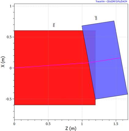
The associated beam envelopes are given below.
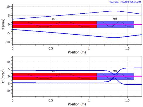
If your ouptut frame is not correctly defined in SUPERPOSE_MAP_OUT, positions and angles shifts are applied at the end of the calculation in the superposed field_map.
Using: SUPERPOSE_MAP_OUT 1573.29 170.0 0 0 0 -11.0
Instead of: SUPERPOSE_MAP_OUT 1573.29 164.27 0 0 0 -9.59023

Positioning of field maps
Each individual element, described by a field map, is associated to a FIELD_MAP keyword:
FIELD_MAP xxxx L θ R kb ke Ke Ka Filename
It is possible to place the field map with any shifted position or/and orientation relatively to the reference frame. The principle is to give the coordinates of the field map origin along with the angle of its frame in the reference frame.
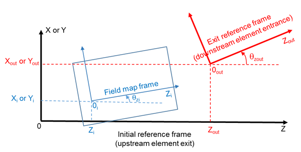
Let's (0, X, Y, Z) be the origin and the axes of the initial reference frame, at the exit of the upstream element, and (0i, Xi, Yi, Zi) those of the frame of the field map i. In order to place the field map i as indicated in the figure, use the command SUPERPOSE_MAP before the FIELD_MAP command as following:
SUPERPOSE_MAP Zi Xi Yi θZi θXi θYi
Pay attention to the order of parameters!
The lengths are in meter and the angles in degree.
Several field maps can be superimposed in the same space, in any order.
In fact, when the SUPERPOSE_MAP commands are used alone, only the parameter Zi is effective. For the other parameters to be taken into account, those commands must preceded by the SUPERPOSED_MAP_OUT command. The latter can also be used for defining an exit reference frame that is different from the initial one. This is particularly useful in case one of the field maps is a dipole. The principle is the same as for the field map frame. In order to place the exit reference frame as indicated in the figure, use the command SUPERPOSE_MAP_OUT as following:
SUPERPOSE_MAP_OUT Zout Xout Yout θZout θXout θYout
Notice that this last command, SUPERPOSE_MAP_OUT, must be used ahead all the SUPERPOSE_MAP commands.
To summarize, the positioning of field maps can be done with the typical commands:
SUPPERPOSE_MAP_OUT ………..
.
.
.
SUPPERPOSE_MAP …………
FIELD_MAP ………….
SUPPERPOSE_MAP …………..
FIELD_MAP ………..
.
.
.
DRIFT ………….
Note that when the SUPERPOSE_MAP_OUT command is used, the reference trajectory is the one linking properly, with the proper deviation, the initial reference frame to the exit one. In graphic representations such as for beam envelope, this reference trajectory is a straight line placed at axis origin. This is what is classically done in accelerator physics.
In order to check if the exit reference frame is correctly positioned as regard to the field map(s) or not, add a drift of enough length at the end of the structure. If it is correct, then the reference trajectory would not present any discontinuity neither in position nor in angle when passing from the field map to the drift.
In order to see the reference trajectory in the field map(s) with its real deviations and positions (and not a straight line), don't use the SUPERPOSE_MAP_OUT command, while keeping the SUPERPOSE_MAP commands. In this case, only the Zi are taken into account and all the other parameters are ignored. So this is only useful when all the maps are aligned with same X, Y, q parameters. Then the beam can be made entering the field map(s) with right X, Y, q parameters by using the Beam Center shifts available at the "Twiss parameters" button of the "Main" tab.
Notice that in all cases, the "Field Map Viewer" will take into account only the Zi parameters and not the other parameters.
|
Mnemonic |
Parameter |
Definition |
|
MULTIPOLE |
Order |
Multipole order |
|
|
L |
Field map length (mm) |
|
|
Nstep |
Number of step along x & y direction |
|
|
field |
Magnetic or electic field on pole (T or MV/m) |
|
|
R |
Aperture (mm) |
|
|
Lsol |
Physical length (mm) of solenoid (Order=0) |
|
|
Zstep Elec |
Number of step for solenoid case (Order=0) 0: Magnetic field map, 1:Electrique field map |
Attention to the TraceWin gradient definition.
The mutipole element generates a 2D (x, y) static magnetic field map file whose steps sizes are: dx = dy = 2.R/Nstep. The step along z direction is defined by TraceWin calculation step. The simulation is made in this field map. Be aware that 2.R/Nstep must be much lower than the beam size.
Order parameter sets the order of the multipole field:
- Order = 0: (Special mode) for solenoid field map (Br(r,z) & Bz(r,z)),
- Order = 1: for dipole,
- Order = 2: for quadrupole,
- Order = 3: for sextupole,
- Order = 4: for octupole,
- …
L is the field map length along z direction.
Nstep defines the number of steps in the generated field map.
B is the magnet
SUPERPOSE_MAP command can be used with this element.
Change element parameters:
Add or change variable, (including or not math expressions)
Move diagnostics in field map element
RFQ:
Lattice commands:
Matching commands:
Minimize beam envelope variation
Errors:
Set of field map
Apply phase error to synchronous phase
Read a multiparticle output file
Magnetic or electric static field
Change transverse beam centroid
Change structure frequency
FREQ f(Mhz)
FREQ command changes the R.F. frequency of the following structure, the beam frequency is not affected. By default, the RF frequency is the beam frequency defined in the TraceWIN GUI.
VARIABLE name value
Varaible can added or changed at any position in the structure as shown in the example below. Name is case sensitive. Attention in the final structure file (*.dat) written at the end of a run, the variables in the elements will all have been replaced by their values.
VARIABLE Gr1 100.0
VARIABLE Gr2 150.0
VARIABLE Apert 35.0
DRIFT 10 10
QUAD 56 Gr1 25
DRIFT 10 10
QUAD 56 Gr1 Apert
DRIFT 10 10
QUAD 56 Gr2 25
DRIFT 10 10
QUAD 56 Gr2 25
DRIFT 10 10
VARIABLE Gr1 120.0
QUAD 56 Gr1 25
END
Mathematical expressions containing the usual mathematical operators (+,-,/,*,^,%) and standard mathematical functions can be implemented when at least one variable is used, as in the following examples:
(The following math functions are supported: abs, acos, asin, atan, atan2, ceil, cos, cosh, exp, floor, ln, log, log10, pow, sin, sinh, sqrt, tan, tanh, fac)
VARIABLE VA1 0.11
VARIABLE VA2 0.22
DRIFT VA1 10 OK
DRIFT 2*VA1 10 OK
DRIFT cos(VA1) 10 OK
DRIFT cos(VA1+VA2+0.1) 10 OK
DRIFT cos(VA1 +VA2+0.1) 10 NOT_OK (because space chars in the equation string are not allowed)
DRIFT sqrt(0.2*VA1+0.1) 10 OK
DRIFT sqrt(0.2+0.1) 10 NOT_OK (because there is no variable)
DRIFT sqrt(0.2*VA1+0.1) 10*VAR2 OK
An ADJUST command placed on a variable will not change the variable but the result of the expression, so this variable will not be changed on the other locations where it is located (see following example).
VARIABLE VA1 0.11
ADJUST 1
DRIFT VA1 10 drift length=0.11 value will be adjsuted
DRIFT 2*VA1 10 drift length will be set to 2*0.11, even after adjustment.
DOUBLET_START
DOUBLET_END
When ‘Set doublet with the same gradient’ option from “Main’ page is selected, the quadrupoles of doublet located in the same machine period are set to same gradient. Both command ‘DOUBLET_START’ and ‘DOUBLET_END’ allows to control the zones where are applied this options.
LATTICE n1 n2
LATTICE command defines the periodic focusing lattices, n1 is the number of element per basic lattice, n2 is the number of lattice per macro-lattice (usually 1). The number of element per macro-lattice is then n1×n2. The basic lattice is used for set the phase advances according to SET_ADV commands. The macro-lattice is used for the phase advance calculation and corresponding matching. All following elements are considered as part of the next lattices until reaching the commands LATTICE_END or END.
The following elements are not included in lattice element counting:
· DIAG_XXX,
· APERTURE,
· THIN_STEERING.
LATTICE_END
LATTICE_END command ends the periodic focusing lattices.
END
END command ends a structure file (*.dat) description (compulsory).
SET_ADV kx0t ky0t
The SET_ADV command sets the zero-current horizontal phase advance to kxot and the zero-current vertical phase advance to kyot.
By default, without kyot value, kyot = kxot.
The periodic focusing lattices structure has to be defined by using the command LATTICE and LATTICE_END, in order to indicate the number of lattice and the number of element per lattice.
The zero-current transverse phase advance law can be imposed in two ways:
When the option “Use phase advance definition” of “Main” page is checked, TraceWin imposes the zero-current transverse phase advance law describe in the Sigma0 file. This file is editable in the “Main” page
If the option “Use phase advance definition” is unchecked that means you have to use the commands SET_ADV in you data file in order to describe your phase advance law.
;FODO lattices in a DTL tank
;Tank 1
LATTICE 2 1
SET_ADV 30
DTL_CEL 87.5277 28 28 0.00548673 71.3977 -71.6524 74699.4 -50 10 0 0.102751 0.723252 -0.475485 -0.194532
DTL_CEL 87.9518 28 28 0.0080072 -71.6524 71.9632 76721.8 -49.5 10 0 0.103248 0.726628 -0.470582 -0.195991
DTL_CEL 88.3919 28 28 0.0112292 71.9632 -72.2903 79282.7 -49 10 0 0.103764 0.734598 -0.458632 -0.197949
DTL_CEL 88.8487 28 28 0.0144758 -72.2903 72.5931 81864.3 -48.5 10 0 0.104299 0.742159 -0.447189 -0.199371
DTL_CEL 89.3222 28 28 0.0177645 72.5931 -72.9101 84484.9 -48 10 0 0.104853 0.74948 -0.436027 -0.200384
DTL_CEL 89.8133 28 28 0.0212224 -72.9101 73.1977 87251.7 -47.5 10 0 0.105428 0.757488 -0.423767 -0.201319
DTL_CEL 90.3217 28 28 0.0245936 73.1977 -73.4992 89953.5 -47 10 0 0.106024 0.764331 -0.413161 -0.201532
DTL_CEL 90.8475 28 28 0.0280032 -73.4992 73.7703 92694.2 -46.5 10 0 0.10664 0.770931 -0.402823 -0.201301
DTL_CEL 91.3909 28 28 0.0314415 73.7703 -74.0554 95477.4 -46 10 0 0.107276 0.777317 -0.392802 -0.200986
SET_ADV 60
DTL_CEL 91.952 28 28 0.0349097 -74.0554 74.3058 98302.2 -45.5 10 0 0.107934 0.783481 -0.38306 -0.200411
DTL_CEL 92.5298 28 28 0.0379774 74.3058 -74.5691 100888 -45 10 0 0.108611 0.787243 -0.377176 -0.2003
DTL_CEL 93.124 28 28 0.0410704 -74.5691 74.8056 103520 -44.5 10 0 0.109308 0.790922 -0.371402 -0.200107
DTL_CEL 93.7349 28 28 0.0442596 74.8056 -75.056 106233 -44 10 0 0.110024 0.794763 -0.365289 -0.199539
DTL_CEL 94.3626 28 28 0.0473999 -75.056 75.2835 108961 -43.5 10 0 0.11076 0.798277 -0.35973 -0.199184
DTL_CEL 95.0078 28 28 0.0507833 75.2835 -75.5255 111880 -43 10 0 0.111516 0.802715 -0.352626 -0.198381
DTL_CEL 95.6703 28 28 0.0539705 -75.5255 75.7413 114710 -42.5 10 0 0.112293 0.80606 -0.347306 -0.197902
DTL_CEL 96.3499 28 28 0.0571744 75.7413 -75.9704 117592 -42 10 0 0.11309 0.809328 -0.342081 -0.197341
DTL_CEL 97.0469 28 28 0.0603973 -75.9704 76.1784 120527 -41.5 10 0 0.113907 0.812524 -0.336963 -0.196748
DTL_CEL 97.7612 28 28 0.0636044 76.1784 -76.3982 123492 -41 10 0 0.114744 0.815493 -0.332338 -0.196611
SET_ADV 40
DTL_CEL 98.4937 28 28 0.0670821 -76.3982 76.5998 126672 -40.5 10 0 0.115603 0.819426 -0.325941 -0.195469
DTL_CEL 99.244 28 28 0.0703571 76.5998 -76.8124 129777 -40 10 0 0.116483 0.822424 -0.321067 -0.19464
DTL_CEL 100.013 28 28 0.0738459 -76.8124 77.0048 133061 -39.5 10 0 0.117384 0.826103 -0.315053 -0.193443
DTL_CEL 100.8 28 28 0.0771374 77.0048 -77.209 136276 -39 10 0 0.118307 0.828909 -0.31049 -0.192635
DTL_CEL 101.604 28 28 0.0804404 -77.209 77.395 139551 -38.5 10 0 0.11925 0.831652 -0.306016 -0.191796
DTL_CEL 102.428 28 28 0.0839794 77.395 -77.5934 143023 -38 10 0 0.120216 0.835125 -0.30028 -0.190411
DTL_CEL 103.271 28 28 0.0875319 -77.5934 77.7738 146561 -37.5 10 0 0.121204 0.838521 -0.29462 -0.188871
DTL_CEL 104.132 28 28 0.0908581 77.7738 -77.9644 150025 -37 10 0 0.122213 0.841052 -0.290457 -0.187938
LATTICE_END
END
“LATTICE 2 1” defines the periodic focusing lattices, 2 is the number of element per lattice (2 DTL cell), 1 is the number of lattice per macro-lattice (generally 1). And TraceWin imposes a phase advance linear continuity between each “SET_ADV” command. This linear continuity can be per lattice or per meter according to the option “Linear phase advance per meter” of the “Main” page. This option is very useful, if you have lattice length discontinuity in order to keep continuity in the phase advance law per meter. TraceWin calculates the quadrupole gradients to obtain the asked zero-current phase advance law, using the lattice transfer matrix.
Warning: it is not always possible to find the required quadrupole gradients.
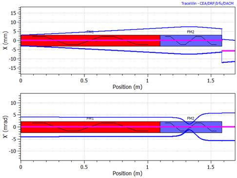
MATCH_FAM_GRAD fn, n, 1/0
MATCH_FAM_FIELD fn, n
MATCH_FAM_PHASE fn, n
MATCH_FAM_LFOC fn, n
MATCH_FAM_LENGTH fn, n
fn is the family or section number and n is the matching element number. When one of these commands precedes an element, it is used (modified) to match the section fn. For example, if two independent cavities are needed to match the beam at the entrance of a section two commands “MATCH_FAM_FIELD” or “MATCH_FAM_PHASE” or “MATCH_FAM_LFOC”, with different matching element numbers n, have to be placed before these cavity entries. But if these two cavities must have the same field, they must have the same matching element number n. If you need for the matching five different quadrupoles and 2 different cavities, then the last command “MATCH_FAM…” must have n = 7. All combinations are possible. You can use the number of quadrupole, the number of cavity and the number of quadrupole or cavity coupled, you want. The coupled elements are not necessarily consecutive. Two examples are presented below. These commands can also be used to match the beam at the entrance of the linac. The only constraint about the family numbers fn is to have a different number per matching family, you can use for example 5,4,8,1...If you set n=0 in each comment of a matching, TraceWin sets automatically a different number for each command, but no coupling is possible between elements.
New (10/09/2012): The third parameter, (0/1), of the command "MATCH_FAM_GRAD" is used for "DTL_CEL" elements to make a difference between the first half quadrupole (0 by default) and second one (1).
MATCH_FAM_GRAD: the quadrupole gradient is adjusted.
MATCH_FAM_FIELD: the field is adjusted.
MATCH_FAM_PHASE: the synchronous phase is adjusted.
MATCH_FAM_LFOC: the longitudinal focalization is adjusted by moving the field and the synchronous phase and the energy gain is kept.
MATCH_FAM_LENGTH: the element length is adjusted.
TraceWin is able to match the beam at the entrance of the linac or between the different sections. In these two cases the criterion for a good matching is either keep the longitudinal and transverse phase advances as smooth as possible or have at the input and the output lattice the same Twiss parameters (taking into account the acceleration parameters.
TraceWin is also able to impose Twiss parameters at a position in the linac. In this case you have to insert a SET_TWISS command behind the matching commands.
These three processes are named “Optimization”, and can be stop by using the menu “Stop”.
To make the optimization of the beam at the entrance of the linac or between the different sections, TraceWin calculates the phase advance on N lattices, using the option “Nbr of phase advance period to smooth” of “Matching” page “. The choice of the criterion (Twiss parameter or smooth phase advances) depends of this option. If the number of lattice is too small (below 6) or if the number of lattice to optimize is set to 0, the Twiss criterion is used. You can watch the optimization process by plotting the phase advance chart, “Beam” and starting the “Synch.” option in the chart. The results of the optimizations can be found in the Results file. The optimization automatically stops when the criterion reaches “Max. Number of iteration” defined in the “Matching” page, but it can be stopped before in the menu “Stop/Optimize”. During a matching some other criterions can be included in order to control the beam size, the beam separation, the beam transverse position or the beam emittance growth...(See matching commands) In this case all the different criterions are added.
Phase advance criterion: ![]() With
With ![]()
With M=2 for DC beam (x,y) or M=3 for bunched beam (x,y,z), and N is the number of lattice to optimize. σt,φ is in °/m.
See also the phase advance definition and setting
If the option “Matching with family & Twiss commands” of page “Matching” is checked, TraceWin changes some quads and cavities strength or element lengths pointed by “MATCH_FAM…” commands, in order to match the beam between two sections. The syntax is not always very easy to use because it has been defined in order to be able to represent most of the cases. Some examples are shown below to help you and if you meet some difficulties yet, send an Email with your data file attached to the authors.
Matching line calculation between a RFQ and a 352 MHz DTL. Two 704MHz buncher cavities and 4 quadrupoles are used in order to match the beam to the structure. A command SET_SIZE_MAX has been include in order to try to reduce the beam size. To help the matching optimization two drift lengths are adjusted by using the command “MATCH_FAM_LENGTH”.
; ***** RFQ-DTL Matching line ******
DRIFT 1e-05 10
FREQ 704
SET_SIZE_MAX 0.025 25 4.5 4.5 25 1
DRIFT 20 10
MATCH_FAM_GRAD 1 0
QUAD 56 55.9938 10
MATCH_FAM_LENGTH 1 0
DRIFT 58.85 10
MATCH_FAM_FIELD 1 0
GAP 251000 -90 10 0 0 0 0 0 0 0
DRIFT 58.85 10
MATCH_FAM_GRAD 1 0
QUAD 56 -56.1374 10
MATCH_FAM_LENGTH 1 0
DRIFT 50.0 10
MATCH_FAM_GRAD 1 0
QUAD 56 62.7152 10
DRIFT 58.85 10
MATCH_FAM_FIELD 1 0
GAP 282000 -90 10 0 0 0 0 0 0 0
DRIFT 58.85 10
MATCH_FAM_GRAD 1 0
QUAD 56 -56.5712 10
DRIFT 70 10
FREQ 352
QUAD 28 71.3977 10
; ***************** DTL *****************
LATTICE 2 1
SET_ADV 46
DTL_CEL 87.5277 28 28 0.00548673 71.3977 -71.6524 74699.4 -50 10 0 0.102751 0.723252 -0.475485 -0.194532
DTL_CEL 87.9518 28 28 0.0080072 -71.6524 71.9632 76721.8 -49.5 10 0 0.103248 0.726628 -0.470582 -0.195991
DTL_CEL 88.3919 28 28 0.0112292 71.9632 -72.2903 79282.7 -49 10 0 0.103764 0.734598 -0.458632 -0.197949
DTL_CEL 88.8487 28 28 0.0144758 -72.2903 72.5931 81864.3 -48.5 10 0 0.104299 0.742159 -0.447189 -0.99371
DTL_CEL 89.3222 28 28 0.0177645 72.5931 -72.9101 84484.9 -48 10 0 0.104853 0.74948 -0.436027 -0.200384
DTL_CEL 89.8133 28 28 0.0212224 -72.9101 73.1977 87251.7 -47.5 10 0 0.105428 0.757488 -0.423767 -0.201319
DTL_CEL 90.3217 28 28 0.0245936 73.1977 -73.4992 89953.5 -47 10 0 0.106024 0.764331 -0.413161 -0.201532
…
..
.
The calculation result is the following:
The first line result contains the 4 quadrupole gradients in T/m, the second is the cavity field corrections and the last the drift lengths in mm.
Matching_Between_Section_0_to_1
56.3399 -56.1173 62.8806 -56.4843
0.934963 0.991466
0.00834559 0.000887792 0.0294733 0.0874924
Matching line calculation between a two super conducting cavity families by adjusting the synchronous phases of the last cavities of the first family and the first cavities of the second family. Four quadrupoles are also adjusted in order to match the beam.
..…
DRIFT 325 100
QUAD 400 10 100
DRIFT 400 100
QUAD 400 -10 100
DRIFT 950 100
NCELLS 1 5 0.6579000 1.11349e+07 -12.331 100 0 0.1801715 0.2934260 -10.0848222 14.7245834 …
DRIFT 475 100
NCELLS 1 5 0.6579000 1.11616e+07 -10.584 100 0 0.1801715 0.2934260 -10.1057623 14.7737516 …
DRIFT 475 100
NCELLS 1 5 0.6579000 1.11873e+07 -8.890 100 0 0.1801715 0.2934260 -10.1259198 14.8211363 …
DRIFT 625 100
SET_ADV 70
DRIFT 325 100
MATCH_FAM_GRAD 8 1
QUAD 400 10 100
DRIFT 400 100
MATCH_FAM_GRAD 8 2
QUAD 400 -10 100
DRIFT 950 100
MATCH_FAM_PHASE 8 3
NCELLS 1 5 0.6579000 1.12121e+07 -7.248 100 0 0.1801715 0.2934260 -10.1453288 14.8668118 …
DRIFT 475 100
MATCH_FAM_PHASE 8 3
NCELLS 1 5 0.6579000 1.12361e+07 -5.657 100 0 0.1801715 0.2934260 -10.1640222 14.9108503 …
DRIFT 475 100
MATCH_FAM_PHASE 8 3
NCELLS 1 5 0.6579000 1.12593e+07 -4.114 100 0 0.1801715 0.2934260 -10.1820316 14.9533216 …
DRIFT 625 100
LATTICE_END
DRIFT 1187.35 100
; Second superconducting family
LATTICE 13 1
SET_ADV 85
DRIFT 325 100
MATCH_FAM_GRAD 8 4
QUAD 500 10 100
DRIFT 400 100
MATCH_FAM_GRAD 8 5
QUAD 500 -10 100
DRIFT 975 100
MATCH_FAM_PHASE 8 6
NCELLS 1 5 0.8458000 1.14453e+07 -94.435 100 0 0.1560511 0.2270898 -10.0611253 13.2916014 …
DRIFT 525 100
MATCH_FAM_PHASE 8 6
NCELLS 1 5 0.8458000 1.14816e+07 -92.773 100 0 0.1560511 0.2270898 -10.0883587 13.3415267 …
DRIFT 525 100
MATCH_FAM_PHASE 8 6
NCELLS 1 5 0.8458000 1.15177e+07 -91.116 100 0 0.1560511 0.2270898 -10.1153599 13.3910179 …
DRIFT 525 100
MATCH_FAM_PHASE 8 6
NCELLS 1 5 0.8458000 1.15536e+07 -89.464 100 0 0.1560511 0.2270898 -10.1421056 13.4400346 …
DRIFT 650 100
DRIFT 325 100
QUAD 500 10 100
DRIFT 400 100
QUAD 500 -10 100
DRIFT 975 100
…
TraceWin sets Twiss parameter to the entrance of a RFQ. To impose Twiss parameter in your structure by adjusting elements you have to use the same “MATCH_FAM…” commands, but a SET_TWISS command has been put in front of the element where you want to impose Twiss parameters at its output. The first parameter of SET_TWISS and “MATCH_FAM…” commands is the family or the section number.
..
…
DRIFT 50.1 100
MATCH_FAM_FIELD 1 0
GAP 154335 -90 100 0 0
DRIFT 50.1 100
MATCH_FAM_LENGTH 1 0
DRIFT 60 100
MATCH_FAM_GRAD 1 0
QUAD 60 16.9089 100
MATCH_FAM_LENGTH 1 0
DRIFT 40 100
DRIFT 20 100
MATCH_FAM_GRAD 1 0
QUAD 60 -16.9089 100
DRIFT 50.1 100
MATCH_FAM_FIELD 1 0
GAP 154335 -90 100 0 0
DRIFT 50.1 100
DRIFT 20 100
MATCH_FAM_GRAD 1 0
QUAD 60 16.9089 100
MATCH_FAM_LENGTH 1 0
DRIFT 40 100
DRIFT 20 100
APERTURE 2.7 2.9 1
FREQ 352.21
DRIFT 0.00001 10
RFQ_CELL 120000 4.96362 0 1 109.954 -60 3
RFQ_CELL 120000 4.96362 0.114946 1.13305 27.4884 -60 4
SET_TWISS 1 -1.5440 0.2462 0.7924 0.1898 -0.0754 0.9523 0 0 0 0 0 0
RFQ_CELL 120000 4.96362 0.114946 1.13305 27.4884 -60 2
RFQ_CELL 120000 4.96362 0.115356 1.13354 27.5261 -60 -2
RFQ_CELL 120000 4.96362 0.115799 1.13406 27.567 -59.9802 2
RFQ_CELL 120000 4.96362 0.116304 1.13465 27.611 -59.9208 -2
RFQ_CELL 120000 4.96362 0.116874 1.13532 27.6552 -59.822 2
RFQ_CELL 120000 4.96362 0.117509 1.13609 27.6995 -59.6843 -2
RFQ_CELL 120000 4.96362 0.118213 1.13692 27.7441 -59.5081 2
RFQ_CELL 120000 4.96362 0.118987 1.13786 27.789 -59.2943 -2
RFQ_CELL 120000 4.96362 0.119833 1.13888 27.8343 -59.0435 2
RFQ_CELL 120000 4.96362 0.120755 1.13999 27.8799 -58.7569 –2
…
..
.
4 quadrupoles and 2 cavities are used to match the beam between section 1 and 2. The longitudinal matching is done by a cavity field modification. This is the simplest case.
LATTICE 7 1 «section 1»
DRIFT 100 100
MATCH_FAM_GRAD 1 1
QUAD 150 10 100 «first quadrupole used for matching »
DRIFT 178.56 100
MATCH_FAM_GRAD 1 2
QUAD 150 -10 100 «second quadrupole used for matching»
DRIFT 488.64 100
MATCH_FAM_FIELD 1 3
GAP 2.94577e+06 -30.5122 100 «first cavity used for matching, the field is adjusted»
DRIFT 722.08 100
LATTICE 9 1 «section 2»
DRIFT 150 100
MATCH_FAM_GRAD 1 4
QUAD 350 10 100 «third quadrupole used for matching»
DRIFT 100 100
MATCH_FAM_GRAD 1 5
QUAD 350 -10 100 «fourth quadrupole used for matching»
DRIFT 935.126 100
MATCH_FAM_FIELD 1 6
GAP 3.04084e+06 -30.5122 100 «second cavity used for matching, the field is adjusted»
DRIFT 1385.81 100
GAP 3.07847e+06 -30.5122 100
DRIFT 729.063 100
4 quadrupoles and 4 cavities are used for the matching between section 1 and 2. The longitudinal matching is done by a cavity phase adjustment. Here, the cavities are coupled 2 by 2.
LATTICE 8 1 «section 1»
…
DRIFT 100 100
MATCH_FAM_GRAD 1 1
QUAD 150 10 100 «first quadrupole used for matching »
DRIFT 178.56 100
MATCH_FAM_GRAD 1 2
QUAD 150 -10 100 «second quadrupole used for matching»
DRIFT 488.64 100
MATCH_FAM_PHASE 1 3
GAP 2.94577e+06 -30.5122 100 «first cavity used for matching, the phase is adjusted. n=3 ».
MATCH_FAM_PHASE 1 3
GAP 2.94577e+06 -30.5122 100 «second cavity used for matching. It will conserve the same phase as the first cavity. n=3 »
DRIFT 722.08 100
LATTICE 10 1 «section 2»
DRIFT 150 100
MATCH_FAM_GRAD 1 4
QUAD 350 10 100 «third quadrupole used for matching»
DRIFT 100 100
MATCH_FAM_GRAD 1 5
QUAD 350 -10 100 «fourth quadrupole used for matching»
DRIFT 935.126 100
MATCH_FAM_PHASE 1 6
GAP 3.04084e+06 -30.5122 100 «third cavity used for matching, the phase is adjusted. n=6 ».
DRIFT 1385.81 100
MATCH_FAM_PHASE 1 6
GAP 3.04084e+06 -30.5122 100 «fourth cavity used for matching, It will conserve the same phase as the third cavity. n=6 »
DRIFT 729.063 100
SET_TWISS fn, αx, βx(mm/mrad), αy, βy(mm/mrad), αz, βz(mm/mrad),kax,kbx,kay,kby,kaz,kbz
The forces of elements pointed with the matching commands "MATCH_FAM_XXX" are adjusted to impose the Twiss parameters given by the "SET_TWISS" command at the output element following the command. More than one command “SET_TWISS” can be used in the same optimization. In this case, use the same fn parameter.
Twiss criterion: 
With ![]()
fn is the section or family number.
βj, γj, αj being the beam Twiss parameters of the space phase xx’, yy’, zz’.
The 6 following parameters “k” are optional, set one to “1” allows to not taking account of the corresponding Twiss parameters
Write “SET_TWISS fn” corresponds to write “SET_TWISS fn 0 0 0 0 0 0 1 1 1 1 1 1”. That disables the SET_TWISS.
SET_POSITION k(m-1), x(mm), x’(mrad), y(mm), y’(mrad)
x, x’, y, y’ are the centroid beam positions imposed at the point where this command appears, k is used in the criterion calculation.
Set position criterion: ![]()
With x(mm), x’(mrad), y(mm), y’(mrad) being the beam centroid transverse positions at the place where the command “SET_POSITION” appears and xo (mm), xo’(mrad), yo (mm), yo’(mrad) being the beam imposed positions.
SET_ACHROMAT k f1 f2 plane
Located after a deviation for instance this command allows to make achromatic the preceding line. k is used to balance the criterion calculation
(f1=1 means set achromatic position).
(f2=1 means set achromatic angle).
If (plane=0) : X or Y or both planes acccoding to bend direction are concerned (default)
If (plane=1) : only X plan is concerned
If (plane=2) : only Y plan is concerned
If (plane=3) : both planes are concerned
Example:
DRIFT 300 100
START_ACHROMAT
EDGE 22.5 500 100 0.45 2.8 50 0
BEND 45 500 0 50 0
EDGE 22.5 500 100 0.45 2.8 50 0
DRIFT 200 100
MATCH_FAM_GRAD 4
QUAD 200 2
DRIFT 200 100
EDGE 22.5 500 100 0.45 2.8 50 0
BEND 45 500 0 50 0
EDGE 22.5 500 100 0.45 2.8 50 0
DRIFT 107 100
SET_ACHROMAT 1.0 1 1
DRIFT 100 100
DRIFT 100 100
END
SET_SIZE_MAX k, N, x(mm), y(mm), θ(°)/z(mm), k2 (0/1)
SET_SIZE_MIN k, N, x(mm), y(mm), θ(°)/z(mm), k2 (0/1)
x, y, θ are the imposed beam size max in the N elements following this command, N, k and k2 is used in the criterion calculation.
When x > x0 set size
max criterion: ![]()
When x < x0 set size min
criterion: ![]()
otherwize vcr = 0
With x(mm), y(mm), θ(°) being the beam maximum sizes in the N elements following the command “SET_SIZE_MAX / MIN”, and xo(mm), yo(mm), θo(°) being the beam imposed sizes. If θ is lower than 0 the longitudinal size used is z(mm). If one of these last parameters is set to 0, no optimization is done on this size and M is reduced by one. If k2=0, the transverses sizes are is calculated without taking account the beam centroid position. If one of the parameters x, y or θ is equal to 0, no optimization is done on this size and M is reduced by one.
The sizes are the effective beam sizes (rms.![]() for bunched beam
or rms.
for bunched beam
or rms.![]() for DC beam)
for DC beam)
SET_SIZE k, x(mm), y(mm), φ(°)/z(mm), k2 (0/1)
x, y, φ are the imposed beam size in the output element following this command, N, k is used in the criterion calculation. If k2=0, the transverses sizes are calculated without taking account the beam centroid position.
Set size criterion: ![]()
With x(mm), y(mm), φ(°) being the beam sizes in the output elements following the command “SET_SIZE”, and xo(mm), yo(mm), ), φ0(°) being the beam imposed sizes. If φ is lower than 0 the longitudinal size used is z(mm). If one of these last parameters is equal to 0, no optimization is done on this size and M is reduced by one.
The sizes are the effective beam sizes (rms*sqrt(5) for bunched beam or rms*sqrt(4) for DC beam)
SET_SEPARATION k, Sx, Sy
Sx0, Sy0 are the centroid beam positions divided by the imposed beam size max at the point where this command appears, k is used in the criterion calculation.
Set separation criterion: ![]()
MIN_EMIT_GROW k, N, ex, ey, ez, f
k and N are used in the criterion calculation.
ex, ey, ez and f are optional: if ex equal to 1 the criterion doesn’t take into account εx beam emittance. That is the same way for ey and ez. f parameter define if the criterion calculation is relative or not (see formula below).
The emittance growth criterion:
§
If (f=1) ![]()
§
If (f=0) ![]() at the command
position
at the command
position
With εxo, εyo, εzo being the beam emittances where this command appears, and εx, εy, εz being the beam emittances after N elements.
STEERER Bx(T) By (T) Bmax 0 coef1(m) coef2(m)
STEERER Ex(V/m) Ey (V/m) Emax(V/m) 1
Its a command not a element (Corresponding element: THIN_STERRING). The magnetic steerer is inserted in the element (magnetic or electric quadrupole, solenoid and field map) placed just after the instruction “Steerer” (keeping the same length). parameters coef1 and coef2 allow to introduce non-linear forces.
![]() And
And ![]()
![]() And
And ![]()
Where x’ and y’ being respectively the horizontal and vertical beam centroid slope.
Used in diagnostic optimization (with ADJUST_STERRER), Bmax and Emax is the maximum limit for Bx, By and Ex, Ey, if it’s greater than zero.
FIELD_MAP case: in field map, kick angle is applied on the full field map length.
The both parameters coef1 and coef2 allow to introduce non-linear forces in the steerer deviation.
coef1 and coef2 units are meter.
- If coef1 is not equal to 0 (SPIRAL2 type steerer):
![]()
![]()
- If coef2 is not equal to 0 (ESS type steerer):
![]()
![]()
With: ![]() see TraceWin gradient definition.
see TraceWin gradient definition.
CHOPPER N, U(V), D(mm), C(mm), p(0/1)
The chopper is inserted in the N elements placed just after the instruction “Chopper” (keeping the same length). U is the voltage between axis and plates and C is the chopper transverse position. ±D is the distance between axis and plates
If (p=0) ![]() and if (p=1)
and if (p=1) ![]()
Where x’ and y’ are respectively the horizontal and vertical beam centroid slope.
ERROR_GAUSSIAN_CUT_OFF cut-off
When the error distribution is defined to Gaussian, this command allow to set a cut-off value.
A new command change this value the following elements concerned by ERROR_XXX commands.
ERROR_BEAM_STAT r(0/1/2), dx(mm), dy(mm), dφ(°), dxp(mrad), dyp(mrad), de(MeV),dEx(%), dEy(%), dEz(%), mx(%), my(%), mz(%), dib(mA), αxx’_min, αxx’_max, βxx’_min(mm/mrad), βxx’_max(mm/mrad), αyy’_min, αyy’_max, βyy’_min(mm/mrad), βyy’_max(mm/mrad), αzdp_min, αzdp_max, βzdp_min(mm/mrad), βzdp_max(mm/mrad)
ERROR_BEAM_DYN
Five kind of error can be set:
Beam displacement: (dx, dy, dr, dxp, dyp, de) The beam input position is not centered.
Emittance growth: (dEx, dEy, dEz) The input beam emittance is increased by a percentage. For DC beam dEz error is applied on the energy spread.
Beam mismatch: (mx, my, mz) The input beam is mismatched by a percentage. A 20 % mismatch in x plane means αx and βx are multiplied by 1.2².
Beam Current error: (dib) Allows to study the effect of the input beam current variation (Ibeam=Ibeam0+dib).
Twiss parameter range: (α_min, α_max, β_min, β_max) The input beam is randomly select in the twiss parameter ranges. The 4 parameters, α_min, α_max, β_min, β_max, must be different of 0 and mismatch parameter m must be equal to 0.
If (r = 0), α_beam = α_min+( α_max- α_min)*k
(k varing from 0 to 1 according to the “Nbr o f step” parameter. If “Nbr_step=4”, k={0, 0.25 ,0.50 ,0.75 ,1)
This command concerns only the input beam. The error distribution depends on the r parameter:
· r = 0, the errors are constant and equal to each value of the command line.
· r = 1, the errors are uniformly distributed (+/-); each value of the command line is the maximum range error.
· r = 2, the errors are Gaussian distribute; each value of the command line is rms value of the distribution.
A Gaussian cut-off can set using SET_GAUSSIAN_CUT_OFF
See also ERROR_STAT_FILE & ERROR_DYN_FILE.
ERROR_QUAD_NCPL_STAT N r(0/1/2/4/5), dx(mm), dy(mm), φx(°), φy(°), φz(°), dG(%), dz(not used) , dG3(%), dG4(%), dG5(%), dG6(%), Nb
ERROR_QUAD_NCPL_DYN
ERROR_QUAD_CPL_STAT
ERROR_QUAD_CPL_DYN
ERROR_QUAD_NCPL_STAT_FILE file
See also ERROR_STAT_FILE & ERROR_DYN_FILE.
New since version 2.16.1.2:
If ERROR_CAV_CPL_XXX and ERROT_QUAD_CPL_XXX commands are located at the same position with the same N parameters then error displacements and rotations applied on cavities and magnet elements will be the same. In this case, error amplitudes are by default defined by ERROR_CAV_CPL_XX.
New since version 2.16.1.0:
Nb parameter allows to limit the number of elements where error are applied, selecting them randomly. For example if you want to move only one quadrupole randomly chosen, this command will do it: ERROR_QUAD_NCPL_STAT 20000 0 0.1 0 0 0 0 0 0 0 0 0 0 0 1
Nb is possible only for _NCPL_ error types.
The N parameter defines the number of elements following the ERROR command that will be affected by these errors. If in this sequence of elements a new command is present, it cancels the previous command from its position to redefine the errors for the next N elements and so one.
dx and dy being respectively the horizontal and vertical magnetic element displacement. dz being the longitudinal shift. φx ,φy, φz being respectively the quadrupole rotation around x, y, z-axis and dG being the gradient amplitude error. dG3, dG4, dG5, dG6 correspond respectively to the sextupole, octupole, decapole, dodecapole gradient errors and concern only QUAD and QUAD_ELE elements. These errors are applied in the N elements following this command, excepted, if a new error command appears. The error distribution depends on the r parameter:
· r = 0, the errors are constant and equal to each value of the command line.
· r = 1, the errors are uniformly distributed (+/-); each value of the command line is the maximum range error.
· r = 2, the errors are Gaussian distribute; each value of the command line is rms value of the distribution.
· r = 4, the errors randomly distributed between 2 values, +MaxErr or -MaxErr. MaxErr is the error amplitude set in the command line.
· r = 5, the errors randomly distributed between 2 values, 0 or MaxErr. MaxErr is the error amplitude set in the command line.
A Gaussian cut-off can set using SET_GAUSSIAN_CUT_OFF
Remark about dG3, dG4, dG5,
dG6 errors: These
errors are only applied on QUAD and QUAD_ELE elements. When the multipole
gradients in the QUAD element are set to zero, then the respective gradient
errors are introduced in terms of quadrupole main field B2, e.g. ![]() ,
, ![]() , etc.. With B2 as magnetic field on pole.
, etc.. With B2 as magnetic field on pole.
The fifth command uses a file to set errors. This file is located by default in structure file (*.dat) path. It contains lines like the following syntax (be careful to Z unit):
Z0(m) r(0/1/2) dx(mm) dy(mm) φx(°) φy(°) φz(°) dG(%) dz(mm), dG3(%) dG4(%) dG5(%) dG6(%)
Z1(m) r(0/1/2) dx(mm) dy(mm) φx(°) φy(°) φz(°) dG(%) dz(mm), dG3(%) dG4(%) dG5(%) dG6(%)
…
Zn(m) r(0/1/2) dx(mm) dy(mm) φx(°) φy(°) φz(°) dG(%) dz(mm) dG3(%) dG4(%) dG5(%) dG6(%)
An interpolation is performed to define errors applied to an element at a given position. It’s not the case for ‘r’ parameter which is defined without interpolation.
A new command “ERROR_QUAD_NCPL_STAT_FILE” without file, put in the *.dat file, stop the action of the preceding similar command.
Be careful: Errors defined by ERROR_QUAD_NCPL_STAT_FILE are added to errors coming from ERROR_QUAD_NCPL_STAT commands.
This error set affects:
- Quadrupole
- Solenoid
- Quadrupole of DTL
- Field map if defined as static magnetic field
PHASE_ERROR_TO_SYNC_PHASE flag
Set to 1 this command allows to apply phase errors directlly to synchronous phase of the cavity instraed to RF phase which is the default case. Set to 0 cancels this feature for all cavities localized after this command.
This command makes errors are canceled and a new synchronous phase setting of the linac are generated.
Phase error amplitudes are defined by ERROR_CAV_NCPL_STAT command, but in this case, errors are transformed in new synchronous phase setting of the linac.
ERROR_CAV_NCPL_STAT N r(0 /±1/2/±3/4/5), dx(mm), dy(mm), φx(°), φy(°), E(%), φ(°), dz(not_used), Nb
ERROR_CAV_NCPL_DYN
ERROR_CAV_CPL_STAT
ERROR_CAV_CPL_DYN
ERROR_CAV_NCPL_STAT_FILE file
See also ERROR_STAT_FILE & ERROR_DYN_FILE.
New since version 2.16.1.2:
If ERROR_CAV_CPL_XXX and ERROT_QUAD_CPL_XXX commands are located at the same position with the same N parameters then error displacements and rotations applied on cavities and magnet elements will be the same. In this case, error amplitudes are by default defined by ERROR_CAV_CPL_XX.
New since version 2.16.1.0:
Nb parameter allows to limit the number of elements where error are applied, selecting them randomly. For example if you want to cut off RF field of a cavity randomly chosen, this command will do it: ERROR_CAV_NCPL_STAT 20000 0 0 0 0 0 -100 0 0 1
Nb is possible only for _NCPL_ error types.
The N parameter defines the number of elements following the ERROR command that will be affected by these errors. If in this sequence of elements a new command is present, it cancels the previous command from its position to redefine the errors for the next N elements and so one.
dx and dy being respectively the horizontal and vertical electric element displacement. dz being the longitudinal shift, φx, φy being respectively the cavity rotation around x, y-axis. E being the field amplitude error. φ being the field phase error. These errors are applied in the N elements following this command, excepted, if a new error command appears. The error distribution depends on the r parameter:
· r = 0, the errors are constant and equal to each value of the command line.
· r = 1, the errors are uniformly distributed (±); each value of the command line is the maximum range error.
· r = -1, the errors are Gaussian distribute; each value of the command line is rms value of the distribution.
· r = 4, the errors randomly distributed between 2 values, +MaxErr or -MaxErr. MaxErr is error amplitude set in the command line.
· r = 5, the errors randomly distributed between 2 values, 0 or MaxErr. MaxErr is the error amplitude set in the command line.
A Gaussian cut-off can set using SET_GAUSSIAN_CUT_OFF
Specail feature for r=2 or r=±3
According to r parameter:
· r = 2, the errors are constant and equal to each value of the command line.
· r = 3, the errors are uniformly distributed (+/-); each value of the command line is the maximum range error.
· r = -3, the errors are Gaussian distribute; each value of the command line is rms value of the distribution.
And the command syntax becomes:
ERROR_CAV_XXX_XXX N r(2/±3), dx(mm), dy(mm), φx(°), φy(°), E(%), kφ(deg/%), dz(mm)
The phase error applied on the cavities is φerr= kφ*Err
In case of coupled error (_CPL_) the field phase and the field amplitude error sign are reversed each new cavity.
The fifth command uses a file to set errors. This file is located by default in structure file (*.dat) path. It contains lines like the following syntax (be careful to Z unit):
Be careful: Errors defined by ERROR_CAV_NCPL_STAT_FILE are added to errors coming from ERROR_CAV_NCPL_STAT commands.
Z0(m) r(0/±1/2/±3) dx(mm) dy(mm) φx(°) φy(°) E(%) φ(°) dz(mm)
Z1(m) r(0/±1/2/±3) dx(mm) dy(mm) φx(°) φy(°) E(%) φ(°) dz(mm)
…
Zn(m) r(0/±1/2/±3) dx(mm) dy(mm) φx(°) φy(°) E(%) φ(°) dz(mm)
An interpolation is performed to define errors applied to an element at a given position. It’s not the case for ‘r’ parameter which is defined without interpolation.
A new command “ERROR_CAV_NCPL_STAT_FILE” without file, put in the *.dat file, stop the action of the preceding similar command.
By default phase errors are applied to RF phase of concerned cavities. The specific command PHASE_ERROR_TO_SYNC_PHASE allows to applied error directly to synchronous phase, but in this case errors are transformed in new synchronous phase setting of the linac.
This error set affects:
- Bunched cavity
- Cavity multi-gap
- DTL (Warning the DTL are only concerns by the field errors)
- Sinus cavity
- Field map if not defined as static magnetic field
ERROR_BEND_NCPL_STAT N, r(0/1/2/4/5), dx(mm), dy(mm), φx(°), φy(°), φz(°), dg(%), dz(mm)
ERROR_BEND_NCPL_DYN
ERROR_BEND_CPL_STAT
ERROR_BEND_CPL_DYN
See also ERROR_STAT_FILE & ERROR_DYN_FILE.
The N parameter defines the number of elements following the ERROR command that will be affected by these errors. If in this sequence of elements a new command is present, it cancels the previous command from its position to redefine the errors for the next N elements and so one.
dx and dy being respectively the horizontal and vertical magnetic element displacement. dz being the longitudinal shift. φx ,φy, φz being respectively the bend rotation around x, y, z-axis and dg being the magnetic field amplitude error. These errors are applied in the N elements following this command, excepted, if a new error command appears. The error distribution depends on the r parameter:
· r = 0, the errors are constant and equal to each value of the command line.
· r = 1, the errors are uniformly distributed (±); each value of the command line is the maximum range error.
· r = 2, the errors are Gaussian distribute; each value of the command line is rms value of the distribution.
· r = 4, the errors randomly distributed between 2 possible values, +MaxErr or -MaxErr. MaxErr is error amplitude set in the command line.
· r = 5, the errors randomly distributed between 2 values, 0 or MaxErr. MaxErr is the error amplitude set in the command line.
A Gaussian cut-off can set using SET_GAUSSIAN_CUT_OFF
This error set affects only magnet bend and edge
Valid only if the BEND element is not cut in several parts.
Warning, the “ERROR_BEND_CPL_X” commands concern only the magnetic field amplitude errors, all other errors (shift, rotation,…) are not couple.
See detail about bend error treatment.
ADJUST N, v, n, min, max, start_step, kn
Red parameters are optional.
This command has to be associated with a Diagnostic elements number N. v, an integer, is the v-th variable to be adjust in the next element list of variable. As an exemple if v=2 and the next element is a quad then the gradient will be adjusted. n (if it’s different from zero) allows to link ADJUST commands each other, therefore, two ADJUST commands with the same n will give the same value to the v variable point. v lower than zero allows to replace both command “ADJUST_DPHASE” and “ADJUST_DFIELD” when v points to phase or field variable.
New in version 2.2.0.16 : The strat_step parameter has been added to select the start step of the fit during optimisation. In other words, the first iteration will be v ± start_step, knowing that the search step may accelerate or decelerate during the optimisation process.
New in version 2.2.1.9: The n parameter allows you to link two variables: If you set the n parameter to the opposite sign, you will get an opposite variation for the linked variables if their initial values are equal. For example, two drifts coupled with (n=1 & n=-1) will keep the same total length. If the initial values are different then they will simply have the same opposite sign value.
New in version 2.20.1.0: The new parameter kn when it is different from 0, allows during a linkage between 2 variables to apply in addition a corrective coefficient, kn. For example, the length of a second drift can be set to half the length of a first drift, which is adjusted.
5 consecutives ADJUST command can be set.
(See Adjust and diagnostic examples)
ADJUST_STEERER N, max, first_step
ADJUST_STEERER_BX N, max, first_step
ADJUST_STEERER_BY N, max, first_step
These commands have to be associated with Diagnostic elements number N and should be placed before a STEERER command. It allows to adjust the horizontal and/or vertical magnetic field steering.
Particular case of steerer adjustment: When the number of steerers corresponds to the number of BPM, no optimization is performed and the resolution of the system is directly made by a matrix inversion
New in version 2.2.0.20: Input beam parameters can be adjusted in order to fit with a set of diagnostic values at different positions of a line
(Example adjusted beam emittances and Twiss parameters at the input of a simulated line in order to obtain the beam sizes measured at different positions with real beam)
ADJUST_BEAM_TWISS N, AlpX_flag, betX_flag, AlpY_flag, BetY_flag, AlpZ_flag, betZ_flag
If flag is set to 1 the selected Twiss parameter will be adjusted, if you want to have alpX=AlpY set alpX_flag=1 and alpY_flag=2, same way for Bet_flag)
ADJUST_BEAM_CENTROID N, X_flag, Xp_flag, Y_flag, Yp_flag, Z_flag, Zp_flag
If flag is set to 1 the selected beam centroid parameter will be adjusted, if you want to have X=Y set X_flag=1 and Y_flag=2, same way for Xp_flag)
ADJUST_BEAM_EMIT N, Ex_flag, Ey_flag, Ez_flag
If flag is set to 1 the selected emittance will be adjusted, if you want to have Ex=Ey set Ex_flag=1 and Ey_flag=2)
ADJUST_BEAM_CURRENT N, I_flag
All “ADJUST_BEAM_XXX” commands must be located in front of the first element. If you are using more than one command of type ADJUS_BEAM, keep to the order shown above. Some elements can be also adjusted in the same matching process.
Beam alignment from a RFQ to a DTL. Two ADJUST commands are associated with two STEERER and with two Diagnostic elements.
DRIFT 0.00001 6.5
DRIFT 56.0 6.5
ADJUST_STEERER 1 «Adjust the steerer inside the following quadrupole »
STEERER -.01 0.01
ERROR_QUAD_NCPL_STAT 1 0 0.1 0.1 0 0 0 0 «Include 0.1mm misalignment and 0.3° rotation errors in the quad »
QUAD 56.0 55.0 6.5
DRIFT 2.15 6.5
DRIFT 58.85 6.5
GAP 180000 -90 6.5
DRIFT 58.85 6.5
ADJUST_STEERER 1 «Adjust the steerer inside the following quadrupole »
STEERER .01 0.01
QUAD 56.0 -55.0 6.5
DRIFT 82.9 6.5
DIAG_POSITION 1 0 0 « Position monitor with x and y position imposed to 0 »
DRIFT 20 6.5
QUAD 56.0 55.0 6.5
DRIFT 58.85 6.5
GAP 210000 -90 6.5
DRIFT 38.85 6.5
QUAD 56.0 -55.0 6.5
DRIFT 54.3 6.5
DIAG_POSITION 1 0 0 « Position monitor with x and y position imposed to 0 »
DRIFT 20.0 6.5
…
You can see the result in the result file. This result is not used in a statistical error study where an adjustment is calculated for each random error distribution.
Diagnostic_1
-0.0661744 -0.0663664 0.0554 0.0458
Triplet adjusting in order to match a beam size
ADJUST 1 2 1 « Quadrupole 1 and 3 are linked, the point variable ‘2’ is the gradient »
QUAD 152 2.14 52
DRIFT 119 52
ADJUST 1 1 0 200 300 « Here, the quadrupole length is adjusted, but the length will keep between (200 & 300) »
QUAD 281 -2.13 52
DRIFT 119 52
ADJUST 1 2 1
QUAD 152 2.0 52
DRIFT 3190 100
APERTURE 2 2 0
DIAG_SIZE 1 2 2
DRIFT 3590 100
DIAG_SIZE 1 4 4
DRIFT 100 100
…
Set achromatic line part from element 3 to achromatic diagnostic position
DRIFT 30 100
DRIFT 30 100
DRIFT 30 100
DRIFT 30 100
EDGE 22.5 500 100 0.45 2.8 50 0
BEND 45 500 0 50 0
EDGE 22.5 500 100 0.45 2.8 50 0
DRIFT 200 100
ADJUST 11 2 1
QUAD 100 -200 20
DRIFT 200 100
ADJUST 11 2 1
QUAD 100 200 20
DRIFT 200 100
ADJUST 11 2 1
QUAD 100 -200 20
DRIFT 200 100
EDGE 22.5 500 100 0.45 2.8 50 0
BEND 45 500 0 50 0
EDGE 22.5 500 100 0.45 2.8 50 0
DRIFT 107 100
DIAG_ACHROMAT 11 3 1 1
DRIFT 100 100
DRIFT 100 100
End
Find the input beam Twiss parameters and emittances given the rms sizes measured at the end of the line.
; Proton @20 MeV, 10 mA
ADJUST_BEAM_CURRENT 99 1
ADJUST_BEAM_EMIT 99 1 2 0 ; Ex=Ey
ADJUST_BEAM_TWISS 99 1 1 1 1 0 0
DRIFT 0 100
DRIFT 100 100
QUAD 100 -15.18 20
DRIFT 200 100
QUAD 100 15.18 20
DRIFT 200 100
QUAD 100 -15.18 20
DRIFT 200 100
DIAG_SIZE 99 2.2 1.6
DRIFT 200 100
DIAG_SIZE 99 2.2 1.6
DRIFT 0 100
END
ERROR_RFQ_CEL_NCPL_STAT N, r(0/1/2), dR(mm), d (mm), E(%),φ(°), TEpe(mm), TEpa(mm), DEpe(mm), DEpa(mm), DELong(mm) TSVerti(mm), TSHori(mm), DSVerti(mm), DSHori(mm), DSLong(m)
ERROR_RFQ_CEL_NCPL_DYN (not implemented yet)
dR is the error for the longitudinal profile, d is the error for the transverse curvature of the electrode, E is the voltage amplitude error. φ being the field phase error (uneffective).
For the transverse plane, TEpe is the perpendicular tilt error by electrode, TEpa is the parallel tilt error by electrode, DEpe is the perpendicular displacement error by electrode, DEpa is the parallel displacement error by electrode, DELong is the a longitudinal displacement error by electrode.
For each segment (block of four electrodes defined with the RFQ_GAP command), TSVerti is the vertical tilt error, TSHori is the horizontal tilt error, DSVerti is the vertical displacement error, DSHori is the horizontal displacement error and DSLong is the longitudinal displacement error.
These errors are applied in the N elements following this command, excepted, if a new error command appears. The error distribution depends on the r parameter:
· r = 0, the errors are constant and equal to each value of the command line (only envelope mode).
· r = 1, the errors are uniformly distributed (±); each value of the command line is the maximum range error.
· r = 2, the errors are Gaussian distribute; each value of the command line is rms value of the distribution.
RFQ is a special element in TraceWin and all these errors are no effect in an envelope calculation except the phase and filed errors.
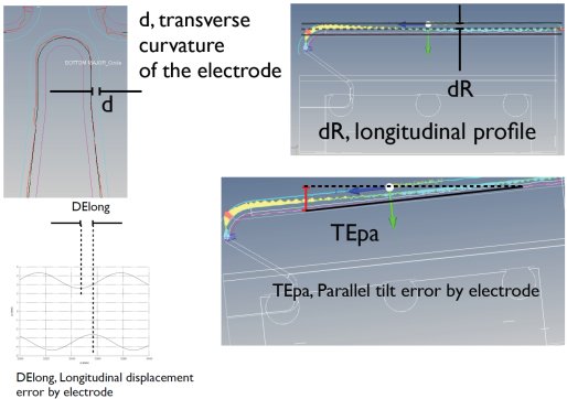
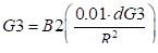
(*) Images provided by Ibon Bustinduy, ESS Bilbao.
PLOT_DST file_out
PLOT_DST_LOST file_out
If file_out parameter is empty, indicate to the multiparticle code to store beam distribution (in the *.plt file) at the end of the next element, otherwise save the beam distribution in file_out as a dst file (.dst extension has to be omitted).
“PLOT_DST_LOST” command allows to include in the dst file, the lost particles.
GAS C, N, P
Only used in multiparticle simulation, this command set the gas pressure parameter until a new command GAS
C is the cross section at 1 MeV (m²), N is the atomic number and P is the pressure (hPa).
You have to select ‘gas stripping’ or ‘gas scattering” in the ‘Multiparticle’ page.
For gas stripping, the actual cross section
used in the simulation is: ![]() , E being the
beam energy in MeV (N is useless).
, E being the
beam energy in MeV (N is useless).
For gas scattering calculations, only N and P are used (C is useless).
Several “gas” commands can be set simultaneously (Max. 9).
MIN_ENV_VARIATION k, N
Minimize the variation of the maximum and minimum transverse beam envelope in magnetic element. For bunched beam, the phase-spread variation is also minimizing in the accelerating elements. The parameter k is a weighting factor for the contribution of this constraint to the overall penalty function and N is the number of element positions over which the constraint applies. The first affected position is the one immediately following the command. Only magnetic and accelerating elements falling within the specified range are affected.
MIN_PHASE_VARIATION k, N, Δθmax
During a matching procedure it is often useful to limit the maximum cavity (synchronous) phase amplitude variation. The parameter k is a weighting factor for the contribution of this constraint to the overall penalty function, θ is the max allowed angle variation in degrees and N is the number of element positions over which the constraint applies. The first affected position is the one immediately following the command. Only cavities falling within the specified range are affected.
![]()
NCPL: means: No Coupled. The errors are individually applied on each element
CPL: means: Coupled. The errors are coupled on the N elements. In other words, a rotation error corresponds to an N elements block rotation.
STAT: means: Static. The effect of these errors can be detected and corrected with appropriate diagnostic and correctors. For example, beam position measurement coupled with steerers can compensate the quadrupole or cavities misalignments. Correction strategy should be known to be able to estimate their impact on beam dynamics
DYN: means: Dynamic. The effect of these errors cannot be measured and then corrected. Fortunately, they have usually lower amplitude than static errors. They are, for example, the vibrations of the elements or the RF field control errors (in phase or amplitude). The knowledge of the correction scheme is not needed to study their statistic impact. They are responsible of orbit oscillations around the corrected orbit (this notion of orbit is also extended in the longitudinal motion).
RFQ_GEOM type N dz
Put this command just before the first RFQ cell.
According to type parameter:
If type = 0: Toutatis generates vane geometry file with 50steps/cell. It’s the default case.
If type = 1: Toutatis reads vane geometry file
Example: RFQ_GEOM 1 c:\my_project\rfq\My_rfq.vane
If type = 2: and N = 0: Toutatis generates vane geometry file with a cell step = dz
Example: RFQ_GEOM 2 0 0.001 for a 1 mm step
If type = 2: and N ≠ 0: Toutatis generates vane geometry file with N step/cell
Example: RFQ_GEOM 2 20
If type = 3: For statistical error study case: (for X cases)
Example: RFQ_GEOM 3 c:\my_project\rfq\My_rfq.vane
Toutatis, for each case, will kook for a RFQ geometry vane file called:
c:\my_project\rfq\My_rfq000001.vane for first run
c:\my_project\rfq\My_rfq000002.vane for second one
…
..
.
c:\my_project\rfq\My_rfq00000X.vane for last one
FOUR_RODS
This option generates electrode profile with varying transverse curvature. By default the transverse curvature is proportional to Ro (four vane type). Put this command just before the first RFQ cell element.
TWOTERMS
This command allows to generate a longitudinal profile (way to modulate) which is governed by the classical 2 terms potential. In case this option is used, only m and a are taken into account, Ro is recomputed. The sinus modulation is the default in case nothing is specified. Put this command just before the first RFQ cell.
RFQ_GAP Lp(m), Lg(m), Sl(m), St(m)
This command defines in a RFQ structure a resonant coupling gap. The position of the command in the data file doesn't matter, if you respect 2 rules: place it before a RFQ cell element, and if you need more than one coupling gap you must avoid to put the new command before the same RFQ cell element. Lp is the longitudinal position of the center of the gap. Lg is gap width. Sl is the half-ellipse size in the beam direction and St is the half-ellipse height in the perpendicular beam direction.
RFQ_GAP_RMS_FFS GapRMS (mm), GapFFS (mm)
This command defined in a RFQ structure, before the first RFQ_CELL element, allows to redefine the front-end gap of the first (GapRMS) and the last (GapFFS) RFQ_CELL (type 3). In Toutatis, these gaps are by defaut defined as ¼ of the front-end cell length. Set GapRMS or GapFFS parameter to 0 to use the Toutatis default values.
SET_OF_MAP
Put this command just before a FIELD_MAP element. This command provides a way to do an error study using a list of field maps.
Used only during statistical error study case: (for X linac)
For each linac, the reference field map will be replaced by a new one named like in the following example:
SET_OF_MAP
LME-Q11 : FIELD_MAP 70 480 0 40 9.174 0 0 0 qpole480_lme
qpole480_lme000001 for first run
qpole480_lme000002 for second one
…
..
.
qpole480_lme00000X for last run
ERROR_STAT_FILE static_error_file.txt
ERROR_DYN_FILE dynamic_error_file.txt
Put this command wherever in the structure file (*.dat), whatever the position, allow to replace static or/and dynamic errors defined by usual error commands (ERROR_QUAD_.XX, ERROR_CAV_XX…), by the values set in the file. Both definition systems cannot coexist, defined errors in files will always dominate. The syntax of the file is identical to the ouput file, “Error_Datas.txt”, containing the applied errors, defined here.
Example:
ERROR_STAT_FILE D:/temp/temp5/Error_Datas_static.txt
ERROR_DYN_FILE D:/temp/temp5/Error_Datas_dynamic.txt
For the special case of a statistical error study: (for X linac)
For each linac, the error file will be replaced by a new one named like in the following example:
D:/temp/temp5/Error_Datas_static000001.txt for first run
D:/temp/temp5/Error_Datas_dynamic000001.txt for first run
D:/temp/temp5/Error_Datas_static000002.txt for second run
D:/temp/temp5/Error_Datas_dynamic000002.txt for second run
…
..
D:/temp/temp5/Error_Datas_static00000X.txt for last run
D:/temp/temp5/Error_Datas_dynamic00000X.txt forlast run
ERROR_SET_RATIO
‘Nstep’ parameter in “Error” page allows to apply progressively the errors from 0% to 100% of the error amplitudes defined by “ERROR_XX” commands. For example “Nstep=4” will perform 4 error studies applying 0% 25% 50% 75% 100% of the maximal error amplitudes.
The command “ERROR_SET_RATIO” allows to user to choose the ratio values.
Example: “ERROR_SET_RATIO 0 0.25 0.75 1.5” will apply 0%, 25% 75% and 150% of the error amplitudes.
The particle file from the page “Main” allows to define the input particle file, but if you want to force the envelope or multiparticle calculation to load a new particle file characteristics (Twiss parameters, current, emittances, centroid) at a given position in the linac, you have to include the command below followed by the full name of the particle file.
READ_DST full_particle_file_name
Warning: This command is read at its position and not like other commands at the end of the following element.
If you choose to run multiparticle code (Partran or Toutatis), you can avoid to run a linac part or even all the linac which has been already computed. Then, you have to indicate to TraceWin, which part doesn’t have to be run, by insert at the beginning of this part the command “READ_OUT” followed by the full name of the Partran or Toutatis output file
READ_OUT full_output_multiparticle_file_name
This command is necessary associated with a READ_DST command (See examples below).
Warning: This command is read at its position and not like other commands at the end of the following element.
The following examples are allowed:
(Where calculation directory is: “D:\temp\temp3\”)
---------------------------------------------------------------------
LBET + RFQ + MEBT: here to avoid to perform the LEBT already calculated, the LEBT is first of all simulated alone and the 3 following file are copied:
- “partran1.out” is copied to “lebt.out”
- “Density_PAR.dat” is copied to “lebt.dat”
- “part_dtl1.dst” is copied to “lebt.dst”
No element before READ_OUT command
No element except, RFQ_CEL, afer READ_DST command
; LEBT
READ_OUT d:\temp\temp3\lebt.out
DRIFT 0 40
DRIFT 10 40
SOLENOID 100 1 40
DRIFT 10 40
SOLENOID 100 1 40
DRIFT 10 40
DRIFT 0 40
READ_DST d:\temp\temp3\lebt.dst
;RFQ
RFQ_CELL 70000 9.94396 0 1 66.9319 -90 3 7.5 1 0 0 0 0
RFQ_CELL 70000 9.94396 6.69068e-05 1.00028 11.1553 -90 4 7.5 1 0 0 0 0
LATTICE 2 1
RFQ_CELL 70000 9.94244 0.000125255 1.00052 11.1553 -90 2 7.5 1 0 0 0 0
RFQ_CELL 70000 9.93848 0.000206589 1.00086 11.1553 -90 -2 7.5 1 0 0 0 0
RFQ_CELL 70000 9.93291 0.000269428 1.00112 11.1553 -90 2 7.5 1 0 0 0 0
RFQ_CELL 70000 9.92632 0.000314328 1.0013 11.1553 -90 -2 7.5 1 0 0 0 0
…
…
RFQ_CELL 70000 8.90751 0.0188169 1.06427 11.1553 -88.3866 -2 7.5 1 0 0 0 0
RFQ_CELL 70000 8.89561 0.0193 1.0658 11.1553 -90.8234 2 7.5 1 0 0 0 0
RFQ_CELL 70000 8.88381 0.0198278 1.06748 11.1553 -89.3208 -2 7.5 1 0 0 0 0
RFQ_CELL 70000 8.87215 0.0203424 1.06911 11.1553 -90.7149 2 7.5 1 0 0 0 0
; MEBT
DRIFT 1 40
QUAD 100 1 40
DRIFT 100 40
QUAD 100 -1 40
DRIFT 100 40
DRIFT 0 40
END
---------------------------------------------------------------------
LBET + RFQ + MEBT: here to avoid to perform the RFQ already calculated, the RFQ is first of all simulated alone and the 3 following file are copied:
- “partran1.out” is copied to “rfq.out”
- “Density_PAR.dat” is copied to “rfq.dat”
- “part_dtl1.dst” is copied to “rfq.dst”
No element after READ_OUT command, except RFQ_CEL
No element before READ_DST command, except, RFQ_CEL
If you have some matching commands in line2, it’s strongly recommended to add at least 5 null drifts just after READ_DST command.
; LEBT
DRIFT 0 40
DRIFT 10 40
SOLENOID 100 1 40
DRIFT 10 40
SOLENOID 100 1 40
DRIFT 10 40
DRIFT 0 40
;RFQ
READ_OUT d:\temp\temp3\lebt.out
RFQ_CELL 70000 9.94396 0 1 66.9319 -90 3 7.5 1 0 0 0 0
RFQ_CELL 70000 9.94396 6.69068e-05 1.00028 11.1553 -90 4 7.5 1 0 0 0 0
LATTICE 2 1
RFQ_CELL 70000 9.94244 0.000125255 1.00052 11.1553 -90 2 7.5 1 0 0 0 0
RFQ_CELL 70000 9.93848 0.000206589 1.00086 11.1553 -90 -2 7.5 1 0 0 0 0
RFQ_CELL 70000 9.93291 0.000269428 1.00112 11.1553 -90 2 7.5 1 0 0 0 0
RFQ_CELL 70000 9.92632 0.000314328 1.0013 11.1553 -90 -2 7.5 1 0 0 0 0
…
…
RFQ_CELL 70000 8.90751 0.0188169 1.06427 11.1553 -88.3866 -2 7.5 1 0 0 0 0
RFQ_CELL 70000 8.89561 0.0193 1.0658 11.1553 -90.8234 2 7.5 1 0 0 0 0
RFQ_CELL 70000 8.88381 0.0198278 1.06748 11.1553 -89.3208 -2 7.5 1 0 0 0 0
RFQ_CELL 70000 8.87215 0.0203424 1.06911 11.1553 -90.7149 2 7.5 1 0 0 0 0
READ_DST d:\temp\temp3\lebt.dst
; MEBT
DRIFT 1 40
QUAD 100 1 40
DRIFT 100 40
QUAD 100 -1 40
DRIFT 100 40
DRIFT 0 40
END
---------------------------------------------------------------------
Line1 + Line2 : here to avoid to perform the Line1 already calculated, the Line1 is first of all simulated alone and the 3 following file are copied:
- “partran1.out” is copied to “line1.out”
- “Density_PAR.dat” is copied to “line1.dat”
- “part_dtl1.dst” is copied to “line1.dst”
No element before READ_OUT command.
If you have some matching commands in line2, it’s strongly recommended to add at least 5 null drifts just after READ_DST command.
; Line1
READ_OUT d:\temp\temp3\line1.out
DRIFT 0 40
DRIFT 10 40
SOLENOID 100 1 40
DRIFT 10 40
SOLENOID 100 1 40
DRIFT 10 40
DRIFT 0 40
READ_DST d:\temp\temp3\line1.dst
; Line2
DRIFT 1 40
QUAD 100 1 40
DRIFT 100 40
QUAD 100 -1 40
DRIFT 100 40
DRIFT 0 40
END
MARKER marker_name
W_P_LIMIT energy_limit(MeV) phase_limit(°)
Works only in tracking mode
If (energy_limit > 0 or phase_limit > 0) then
If | W –Synchonous energy | > energy_limit particle is set as lost
If | P –Synchronous phase | > phase_limit particle is set as lost
If (energy_limit < 0 or phase_limit < 0) then
If | W –beam energy centroid | > | energy_limit | particle is set as lost
If | P –beam phase centroid | > | phase_limit | particle is set as lost
CHANGE_BEAM q ∆WgE ∆WfE ∆WgM ∆WfM ∆z auto_flag(0/1) Φg Φf
q : Change the particle charge state.
∆WgE (eV): shift the linac reference energy (Wg=Wg+∆Wg)in envelope mode
∆WfE (eV): shift the beam energy (Wf=Wf+∆Wf) in envelope mode
∆WgM (eV): shift the linac reference energy (Wg=Wg+∆Wg) in tracking mode
∆WfM (eV): shift the beam energy (Wf=Wf+∆Wf) in tracking mode
∆z(mm): allows to shift the changing point inside a FIELD_MAP element
Φg/f (deg): RFQ output reference and beam absolute phase in envelope mode (normaly identical). A shift can be introduced (Φg - Φf) changing Φf in order to shift the output beam phase in tracking and set it to 0. If phase of RF components of the foolwing linac is relative following Φg can be set to 0 and just adjust Φg to canvel the output bema phase in tracking.
If auto_flag is set to ‘1’ linac referecene energy is automatically set to beam energy
(This command could be extended according to futur needs)
The “CHANGE_BEAM” command is mainly used to make transition betwen TraceWin and Toutatis because both codes don’t use exactly the same way to calculate the output reference and beam energies. Mainly because Toutatis is a ‘t’ code and TraceWin is a ‘z’ code. The command “CHANGE_BEAM” has been implemented to cancel these differences and make more compatible both codes. You just have to follow the procedure below to define the right command parameters.
In input “inp” file of Toutatis code:
- Remove « DatFlag » in the input « inp » file of Toutatis in order to generate input data file “rfq.dat” for TraceWin code.
- Set “theAcceleratedFlag 1”
- Set “theAccuracyFlag 1”
- Run Toutatis
In TraceWin project:
- Use “rfq.dat” file generated by Toutatis as structure file in TraceWin project
- Check TraceWin toutatis options in TraceWin (“Multiparticle” tab-sheet and “Toutatis options”):
- UnCheck “Coase mesh”
- Check “Exclude not accelerated particles”
- Check “Number of step per period” is equal to NStep parameter of “inp” file
- Put the same particle number, beam current and input energy parameters used in “inp” file in TraceWin project.
- In tab-sheet “Matching” select “Calculate input matched beam”.
- In “Multiparticle” tab-sheet -> “Partran Energy and Phase limits”, set 0.1 & 180° in particles excluded from emittance calculation parameters.
- In “Multiparticle” tab-sheet select “Launch Tracking” for “Partran” and “Toutatis”.
- Run project
- In “Charts” tab-sheet have a look on the output phase space distribution for Tracking (Partran). You should have something like following. In “data” tab-sheet, you can find beam absolute phase and energy of envelope simulation.
![]()
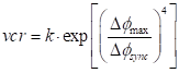
- Put at the end of RFQ structure the command line
CHANGE_BEAM q -26860 -26860 0 0 0 0 75825.949 75827.311
26860 eV corresponds to the difference between the beam energy of the tracking output and that of the envelope.
75825.9° is the envelope output absolute phase
78827.311° is the envelope output absolute phase shifted of 1.362° coming from tracking simulation.
So after this command, the phase and energy of the envelope calculation should be aligned with the tracking results.
Set “q” to your particle charge state, 1 for proton.
- Run another time the project and have a look on the output phase space distribution for Tracking and envelope. You should have something like following (Two or three iterations are sometime necessary):
![]()

So, now both envelope and tracking give the same output energy and output tracking phase is close to 0.
SHIFT dx(mm), dy (mm)
Move the following element.
SHIFT_BEAM dx(mm), dy (mm), dx’(mrad), dy’ (mrad)
Change transverse beam centroid values before the following element.
PARTRAN_STEP step1, step2
Step1 is the new step of calculation per metre; step2 is the new step of space-charge calculation per meter until reaching a new “PARTRAN_STEP” command. The default step1 and step2 value is put in the “Multiparticle” page, see “Partran step of calcul”.
These two step concern only DRIFT and FIELD_MAP elements, all other elements are treated in 2 steps.
SPACE_CHARGE_MESH meshXY, meshZ
Dynamically changes the mesh space mesh for the picnic routine in tracking simulations. No limit is set but the memory requiered can quickly become enormous, as the computation time. Multiple commands can change the mesh at different machine positions.
FIELD Bx(T), By (T), Bz (T) Ex (V/m) Ey (V/m) Ez (V/m)
Add to the following elements a magnetic or electric force until a new command “FIELD” canceling the preceding. In PARTRAN simulation, only the field command of the first element is considering.
![]()
![]()
![]() .
.![]() .
. ![]()
Where x’ , y’ and g being respectively the horizontal and vertical beam centroid slope and the the reduced energy
SET_BEAM_PHASE_ADV k, N, φx(°), φy(°), φz(°)
φx, φy, φz, are the imposed beam phase advance in space charge during N elements from command. k is used in the criterion calculation. The behaviour of this command is unusual because it applies to the entrance of the element where it is placed. So for example if it is localized at element#1 and N is 7, the phase advance is calculated from the input of element#1 to the output of element#7.
Set beam adv criterion: ![]()
With φx(°), φy(°), φz(°) being the beam phase advances in the output elements following the command “SET_BEAM_PHASE_ADV”, and φx0(°), φy0(°), φz0(°), being the imposed beam phase advances. If one of these last parameters is equal to 0, no optimization is done on this phase and M is reduced by one.
SET_BEAM_E0_P0 k, ΔE, Δφ, ke, kp
ΔE and Δφ, are the imposed delta beam energy and phase.
Set beam energy and phase criterion: ![]()
With ΔE0 being the difference between the beam energy and the linac energy (close to 0 in the ideal case without error). And Δφ0 being the difference between the beam phase and the linac phase (close to 0 in the ideal case without error)
ke, kp allow to take into account or no one of both.
SET_BEAM_ENERGY k, Ei
Ei is the imposed beam energy (MeV).
Set beam energy criterion: ![]()
With E being the the beam energy.
SET_SYNC_PHASE
The phase given in an RF element preceded by the SET_SYNC_PHASE command is the synchronous phase of the generatrix particle, rather than the absolute phase (by default). It applies to following elements:
FIELD_MAP
RFQ_CEL
CAVSIN
NCELLS
MIN_FIELD_VARIATION k, N, ΔEmax
During a matching procedure it is often useful to limit the maximum field amplitude variation. The parameter k is a weighting factor for the contribution of this constraint to the overall penalty function, θ is the max allowed angle variation in degrees and N is the number of element positions over which the constraint applies. The first affected position is the one immediately following the command. Only cavities falling within the specified range are affected.
![]()
REPEAT_ELE k, n
Allows to duplicate the following n elements k times. Caution: The associated commands are also repeated except: ‘LATTICE’, ‘LATTICE_END’ and ‘SET_ADV’ one. A ‘REPEAT_ELE’ command cannot include another one.
;Example: 100 times a period.
DRIFT 5 30
DRIFT 5 30
REPEAT_ELE 100 4
LATTICE 4 1
SET_ADV 20
QUAD 100 1530 0
DRIFT 100 30
QUAD 100 -15 30 0
DRIFT 100 30
LATTICE_END
DRIFT 5 30
DRIFT 5 30
END
;Example : Repeat 10 times a quadrupole
DRIFT 5 30
REPEAT_ELE 10 1
QUAD 10 15 30 0
DRIFT 5 30
END
;Example : Divide in 10 steps a dipole with Edge and fringe-field.
EDGE 20 600 40 0 0 25 0
BEND -90 600 0 20 0
EDGE 20 600 40 0 0 25 0
Become
EDGE 20 600 40 0 0 25 0
BEND -9 600 0 20 0
EDGE 0 600 40 1e-12 1e-12 25 0
REPEAT_ELE 8 3
EDGE 0 600 40 1e-12 1e-12 25 0
BEND -9 600 0 20 0
EDGE 0 600 40 1e-12 1e-12 25 0
EDGE 0 600 40 1e-12 1e-12 25 0
BEND -9 600 0 20 0
EDGE 20 600 40 0 0 25 0
SHIFT_IN_FIELD_MAP dz
Using this command in front of diagnostics elements allows overlapping with the following FIELD_MAP. Dz must be greater than 0 and several diagnostics can be used. See following example where 2 diagnostics are localised into 2 supperposed field maps.
DRIFT 100 100
SHIFT_IN_FIELD_MAP 200
DIA1 : DIAG_SIZE 2
SHIFT_IN_FIELD_MAP 360
DIA2 : DIAG_SIZE 5
SUPERPOSE_MAP 0
LME-Q11 : FIELD_MAP 70 480 0 40 9.174 0 0 0 qpole480_lme_25_01_07b
SUPERPOSE_MAP 350
LME-Q11 : FIELD_MAP 70 480 0 40 -9.174 0 0 0 qpole480_lme_25_01_07b
DRIFT 100 100
end
SUPERPOSE_MAP Z0 X0 Y0 θ Z0 θ X0 θ Y0
A FIELD_MAP element already allows to superpose 4 field map types (electrostatic, electrodynamic, magnetic or electric field map). With the “SUPERPOSE_MAP” command, different FIELD_MAP elements can be superposed at different postions Z0 of the reference trajectory.
The optionnals parameter, X0 Y0 θ Z0 θ X0 θ Y0 are required when the following field map curves the reference trajectory (See Field map with curved reference trajectory). Another command is also needed to inform code to output frame.
If you want to use field map aperture or current in case of superposed field map, you have to include a empty field map element a the position 0 including aperture and/or current field map.
;Example: quadrupole inside a solenoid.
DRIFT 5 30
SUPERPOSE_MAP 400
FIELD_MAP 70 100 0 42 -0.3 0 0 0 qpole_field_map_file
SUPERPOSE_MAP 0
FIELD_MAP 70 1000 0 100 -1.3 0 0 0 solenoid_fiedl_map_file
DRIFT 5 30
End
FIELD_MAP_PATH path
Set at the top of the structure file (*.dat), it allows to indicate the directory where is store thefield map file. This path can be absolute of relatice to the project file path. Up to 3 commands can be used, the first valid path will be used.
SUPERPOSE_MAP_OUT Z0 X0 Y0 θ Z0 θ X0 θ Y0
(X0, Y0, Z0) gives to the position in [m], in (X, Y, Z) frame, of the exit point of the simulation in the field map,
(θ X0,
θ Y0, θ Z0) gives the rotation
angles in [°] between the reference trajectory directions at the exit point of
the simulation in the field map ![]() and
and![]()
See Field map with curved reference trajectory chapter or FIELD_MAP element for get more details.
SET_BEAM_PHASE_ERROR Dp(°) RamdomFlag(0/1)
If Dp is equal to zero, this command allows to cancel, phase error coming from preceding elements. The beam phase is not affected by this command, the strategy is to shift all the following cavity RF phases, by the difference between reference design and beam phase observe at the command position. By this way, you have the possibility to uncouple the RF phase of some part of the machine and start a linac part with a new RF phase.
This command cannot correct to phase errors coming from dynamic errors, only static or input beam error can be corrected.
If Dp not equal to zero and RamdomFlag is equel to zero, the RF shift will be increased of Dp value.
If Dp not equal to zero and RamdomFlag is not equal to zero, the RF shift will be increased of a ramdom value between +/-Dp.
This feature allows to each user to develop its own element or diagnostics. A detailed example following explains how to perform it. Use the following ‘my_elemens.cpp’ file and compile it as a dynamic library. This library has be located either in the structure (*.dat) directory or in the executable directory.
/***************************************************************************
main.cpp
Windows -> Dynamic library (dll)
Linux or MacOS -> Dynamic shared object (so, dylib)
-------------------
begin : Wed Dec 1 2010
copyright : (C) 2010 by URIOT Didier
email : duriot@cea.fr
***************************************************************************/
#ifdef _WIN32
#include <windows.h>
#define DLL_EXPORT __declspec(dllexport)
#else
#define DLL_EXPORT
#endif
#include <cmath>
#include <cstdio>
#include <cstdlib>
#include <cstring>
#ifdef __cplusplus
extern "C" {
#endif
//---------------------------------------------------------------------------
//-- MY_ELE - MY_ELE - MY_ELE - MY_ELE - MY_ELE - MY_ELE - MY_ELE -----------
//-- MY_ELE - MY_ELE - MY_ELE - MY_ELE - MY_ELE - MY_ELE - MY_ELE -----------
//---------------------------------------------------------------------------
//
// Syntax in struture.dat file
//
// MY_ELE(my_ele_name) L(mm),R(mm),Nstep,arg3,arg4...arg20
// following functions have to be defined
// - my_ele_name_partran : for the beam tracking treatment
// - my_ele_name_envelope : for the beam envelope treatment
//
// If "my_ele_name" is not defined (MY_ELE target arg2,arg3...arg10)
// following functions have to be defined
// - my_ele_partran : for the beam tracking treatment
// - my_ele_envelope : for the beam envelope treatment
//
// Settings (L, R, Nstep) must be defined
// - Element length (mm)
// - Aperture R (mm): This parameter are only used for plotting, you have to manage yourself the particle losses.
// - Nstep : the element will cut in Nstep part with a space-charge kick each 2 steps
// If Nstep = 0 the number of space-charge kick will be defined by TraceWin according to "step of space-charge" parameter of "Multiparticle" page.
// If Nstep = 1 the element will not be cut in and no space-charge kick will be applied
// - arg3 to arg20 : Free parameters available for user
//
// Below you can find an example (Drift element)
//
// Syntax: MY_ELE(my_drift) L(mm),R(mm),Nstep,arg3,arg4...arg20
// 2 functions habe to be defined
// - my_drift_partran : for the beam tracking treatment
// - my_drift_envelope : for the beam envelope treatment
// You have to compile this example as an dll
// - my_elements.dll (for windows)
// - my_elements.so (for linux)
// - my_elements.dylib (for MacOS)
//
// Commands to compil and link GNU gcc compiler on Windows:
// g++.exe –m64 -Wall -c my_elements.cpp -o my_elements.o
// g++.exe –m64 -shared -Wl my_elements.o -o my_elements.dll
// If you use 32bits TraceWin version replace both –m64 by –m32
// Commands to compil and link GNU gcc compiler on Linux:
// g++ -m64 –fPIC -Wall -c my_elements.cpp -o my_elements.o
// g++ -m64 -fPIC -shared -Wl my_elements.o -o my_elements.so
// If you use 32bits TraceWin version replace both –m64 by –m32
// Commands to compil and link GNU gcc compiler on MAC OS:
// g++ -m64 -Wall -pedantic -c my_elements.cpp -o my_elements.o
// g++ -m64 -Wall -shared -dynamiclib my_elements.o -o my_elements.dylib
// If you use 32bits TraceWin version replace both –m64 by –m32
// MY_ELE Multiparticle (Drift example) [ MY_ELE(my_drift) L(mm), R(mm), Nstep ]
// MY_ELE Multiparticle (Drift example) [ MY_ELE(my_drift) L(mm), R(mm), Nstep ]
int DLL_EXPORT my_drift_partran(double Zs,double *param,int Nele,int npart,double *cord,double *loss,double freq,double mass0,int q,double *ws,double *Ibeam,double *extra_param,char *error_mess)
{
double x,y,xp,yp,z,w,dpsp,r,zzs,bgs,gamma,gams,betas,ds,Aperture;
//
// Zs : Current position in the element (from 0 to Length-Length/Nstep)
// param[1] : Length/Nstep (m)
// param[2] : Aperture (m)
// param[3] : Nstep
// cord : See example
// loss : see example
// freq : beam frequency (Hz)
// mass : Particle mass (eV)
// q : particle charge state
// *ws : reference kinetic energy (eV) (can be modified)
// *Ibeam : Beam current (A) (can be modified)
// error_mess : TraceWin stop and show this error message if this function return 0
// if error_mess!="" and function return 1, this message is print to the standard console without stop TraceWin
ds=param[1];
Aperture=param[2];
strcpy(error_mess,"");
zzs=(*ws)/mass0;
bgs=sqrt(zzs*(2.+zzs));
gams=1.0+zzs;
betas=bgs/gams;
for (int i=0;i<npart;i++) {
if ((int)loss[i]==0) {
x=cord[i*6]; // m
xp=cord[i*6+1]; // rad
y=cord[i*6+2]; // m
yp=cord[i*6+3]; // rad
z=cord[i*6+4]; // m
dpsp=cord[i*6+5]; // dp/p
r=sqrt(x*x+y*y);
if (r>Aperture) loss[i]=Nele; // A particle lost has to be set to Element number
else {
x=x+ds*xp;
y=y+ds*yp;
w=dpsp*betas*betas*gams*mass0+(*ws);
gamma = 1+w/mass0;
z=z+dpsp*ds/(gamma*gamma);
}
cord[i*6]=x;
cord[i*6+2]=y;
cord[i*6+4]=z;
}
}
return(1);
}
//--------------------------------------------------------------------------------------------------------------------------------------------------------------------
// MY_ELE Envelope (Drift example)
// MY_ELE Envelope (Drift example)
int DLL_EXPORT my_drift_envelope(double Zs,double *param,int Nele,double Tmat[][6],double *Bcent,double freq,double mass0,int q,double *ws,double *ibeam,double *extra_param,char *error_mess)
{
//
// Zs : Current position in the element (from 0 to Length-Length/Istep)
// my_ele_envelope is first time called wiht parma[1]=Length (in this case Zs=-10)
// the following calls is performed Istep times for Zs from 0 to Length-Length/Istep (Istep is defined by TraceWin according to "step of calcul" parameter of "Main" page.
// param[1] : Length(m) or Length/Istep (m)
// param[2] : Aperture (m)
// param[3] : Nstep
// cord : See example
// loss : see example
// freq : beam frequency (Hz)
// mass : Particle mass (eV)
// q : particle charge
// *ws : reference kinetic energy (eV) (can be modified)
// *Ibeam : Beam current (A) (can be modified)
// error_mess : TraceWin stop and show this error message if this function return 0
// if error_mess!="" and function return 1, this message is print to the standart console without stop TraceWin
double gams;
double ds=param[1];
strcpy(error_mess,"");
gams = 1+(*ws)/(mass0);
Tmat[0][0]=Tmat[1][1]=1;
Tmat[0][1]=ds;
Tmat[2][2]=Tmat[3][3]=1;
Tmat[2][3]=ds;
Tmat[4][4]=Tmat[5][5]=1;
Tmat[4][5]=ds/(gams*gams);
return(1);
}
//--------------------------------------------------------------------------------
//-- MY_DIAG - MY_DIAG - MY_DIAG - MY_DIAG - MY_DIAG - MY_DIAG - MY_DIAG ---------
//-- MY_DIAG - MY_DIAG - MY_DIAG - MY_DIAG - MY_DIAG - MY_DIAG - MY_DIAG ---------
//--------------------------------------------------------------------------------
//
// Syntax in struture.dat file
//
// MY_DIAG(my_diag_name)(Weight) Diag_number target arg2,arg3...arg10
// Diag_number is the number to associated to ADJUST commands
// “(Weight)” is optional
//
// following functions have to be defined
// - my_diag_name_partran : for the beam tracking treatment
// - my_diag_name_envelope : for the beam envelope treatment
//
// If "my_diag_name" is not defined (MY_DIAG target arg2,arg3...arg10)
// 2 functions are defined
// - my_diag_partran : for the beam tracking treatment
// - my_diag_envelope : for the beam envelope treatment
//
// TraceWin Criteria = pow(target_value - diag_value),2)
//
//
// below you can find an example of a beam position or beam size measurment :
// Syntax: MY_DIAG(my_pos_and_size) target arg2,arg3...arg10
// following functions have to be defined
// - my_pos_and_size_partran : for the beam tracking treatment
// - my_pos_and_size_envelope : for the beam envelope treatment
// You have to compile this example as an dll
// - my_elements.dll (for windows)
// - my_elements.so (for linux)
// - my_elements.dylib (for MacOS)
// Commands to compil and link GNU gcc compiler on Windows:
// g++.exe -m32 -Wall -c main.cpp -o main.o
// g++.exe -m32 -shared -Wl main.o -o my_elements.dll
// If you use 64bits TraceWin version replace both -m32 by -m64
// Commands to compil and link GNU gcc compiler on Linux:
// g++ -m32 –fPIC -Wall -c main.cpp -o main.o
// g++ -m32 –fPIC -shared -Wl main.o -o my_elements.so
// If you use 64bits TraceWin version replace both -m32 by -m64
// Commands to compil and link GNU gcc compiler on MAC OS:
// g++ -m32 -Wall -pedantic -c main.cpp -o main.o
// g++ -m32 -Wall -shared -dynamiclib main.o -o my_elements.dylib
// If you use 64bits TraceWin version replace both -m32 by -m64
// MY_DIAG Multiparticle
// MY_DIAG Multiparticle
int DLL_EXPORT my_pos_and_size_partran(double *diag_value,double *param,int Nele,int npart,double *cord,double *loss,double freq,double mass0,int q,double ws,double Ibeam,double *extra_param,char *error_mess)
{
double x2,x,y,xp,yp,z,dpsp,xmoy;
int ng;
//
// param[1] : target_value
// param[2] : you can use this second parameter to define to diagnostic types
// param[3->8] : free
// diag_value : value of your diagnostic
// cord : See example
// loss : see example
// freq : beam frequency (Hz)
// mass : Particle mass (eV)
// q : particle charge state
// ws : reference kinetic energy (eV) (can be modified)
// Ibeam : Beam current (A) (can be modified)
// error_mess : TraceWin stop and show this error message if this function return 0
// if error_mess!="" and function return 1, this message is print to the standart console without stop TraceWin
strcpy(error_mess,"");
xmoy=x2=0;
ng=0;
for (int i=0;i<npart;i++) {
if ((int)loss[i]==0) {
x=cord[i*6]; // m
xp=cord[i*6+1]; // rad
y=cord[i*6+2]; // m
yp=cord[i*6+3]; // rad
z=cord[i*6+4]; // m
dpsp=cord[i*6+5]; // dp/p
x2+=x*x;
xmoy+=x;
ng++;
}
}
if (param[2]==0) {
xmoy/=ng;
*diag_value=xmoy; // X position (m)
}
if (param[2]==1) {
x2=sqrt(x2/ng);
*diag_value=x2; // X size (m)
}
// sprintf(error_mess,"%lg %d %lg %lg",param[2],ng,x2,*diag_value);
return(1);
}
//--------------------------------------------------------------------------------------------------------------------------------------------------------------------
// MY_DIAG Envelope
// MY_DIAG Envelope
int DLL_EXPORT my_pos_and_size_envelope(double *diag_value,double *param,int Nele,double Bmat[][6],double *Bcent,double freq,double mass0,int q,double ws,double ibeam,double *extra_param,char *error_mess)
{
//
// param[1] : target_value
// param[2] : you can use this second parameter to define to diagnostic types
// param[3->8] : free
// diag_value : value of your diagnostic
// Nele : Element number
// Bmat : Beam matrix 6x6 (x(m), xp(rad, y(m), yp(rad), z(m), dp/p)
// Bcent : beam centroid vector (x(m), xp(rad, y(m), yp(rad), z(m), dp/p)
// freq : beam frequency (Hz)
// mass : Particle mass (eV)
// q : particle charge state
// ws : reference kinetic energy (eV) (can be modified)
// Ibeam : Beam current (A) (can be modified)
// error_mess : TraceWin stop and show this error message if this function return 0
// if error_mess!="" and function return 1, this message is print to the standart console without stop TraceWin
printf("POS ENV\n");
if (param[2]==0) {
*diag_value=Bcent[1]; // X beam position (m)
}
if (param[2]==1) {
*diag_value=sqrt(Bmat[0][0]); // beam size (X); (m)
}
return(1);
}
#ifdef __cplusplus
} // "C"
#endif
EXCITATION_CURVE a0 a1 a2 a3
To set the strength of magnetic element as quadrupole, solenoid or dipole, the field map parameter kb has to be set to amplitude depending of the field defined in the map. It is sometime more convenient to use directly the power supply current when we get the excitation curbe B(I) or G(I). The gradient normalization is calculated at
5% of the bore radius. This command has to be defined at the first occurance of a field map defined by this file name. All following field map using the same file are automatiquely concerned. See following example using quadrupole.
DRIFT 10 100
LME-Q11 : FIELD_MAP 70 480 0 40 5.20 0 0 0 qpole_file ; kb=5.20 -> gradient is not knew directly
DRIFT 10 10
LME-Q12 : FIELD_MAP 70 480 0 40 10.4 0 0 0 qpole_file; kb=10.4 -> gradient is not knew directly
DRIFT 10 100
END
; Here the gradient values depend of the kb parameters and the field amplitudes defined in the qpole_file.

The excitation curbe G(I) can be aproximativement defined as polynome and and its coefficients are used in the commande.
DRIFT 10 100
EXCITATION_CURVE -3.12e-13 7.00e-2 -1.28e-4 -1.08e-19
LME-Q11 : FIELD_MAP 70 480 0 40 40 0 0 0 qpole_file ; kb=40A -> gradient is set 2.59 T/m
DRIFT 10 10
LME-Q12 : FIELD_MAP 70 480 0 40 80 0 0 0 qpole_file ; kb=80A -> gradient is set 4.77 T/m
DRIFT 10 100
END
EXCITATION_CURVE2
Thi second command allows to use all table G(I) data. In this case a file named as the field map name (“qpole_file.gi” in the following example) has to be located with the magnetic field map files. The syntax of the file is show below, the first number indicates the nomber of lines, then first collum is the power supply currant (A) and the second one is the gradient (T/m). A splin interpolator will be used to estimate G(I).
DRIFT 10 100
EXCITATION_CURVE2
LME-Q11 : FIELD_MAP 70 480 0 40 40 0 0 0 qpole_file ; kb=40A -> gradient is set 2.59 T/m
DRIFT 10 10
LME-Q12 : FIELD_MAP 70 480 0 40 80 0 0 0 qpole_file ; kb=80A -> gradient is set 4.77 T/m
DRIFT 10 100
END
|
11 |
|
|
0 |
0,0000 |
|
25 |
1,6813 |
|
50 |
3,3407 |
|
75 |
5,0350 |
|
100 |
6,6783 |
|
125 |
8,3435 |
|
150 |
9,9867 |
|
175 |
11,5855 |
|
200 |
12,9745 |
|
225 |
14,0765 |
|
265 |
15,4146 |
SAVE_DATA data abscissa Envelope/Partran
This command, which may appear up to 10 times in the ‘*.dat’ file (regardless of its position), allows the data defined by the ‘data’ parameter to be saved at the end of a simulation in “data.txt” file name. The ‘abscissa’ parameter allows you to select the abscissa, and the ‘Envelope/Partran’ (0/1) parameter allows you to select data from an envelope or tracking result.
Example: « SAVE_DATA Synchronous_phase 2 0 » save in “Synchronous_phase.txt” file the beam synchronous phase from envelope simulation according to the linac position.
abscissa :
0 : abs="Element#"
1 : abs="Period#";
2 : abs="Position (m)"
3 : abs="W (MeV)"
4 : abs="β"
data :
TPhaseAdv_On_LPhaseAdv graph="Transv. Phase Adv / Long. phase Adv"
Field_Map_Factors graph="Field Map Factors"
Period_length graph="Period length (m)"
Energies graph="Energy (MeV)"
Synchronous_phase graph="Synchronous phase (deg)"
Cavity_power graph="Cavity power (kW)"
Acceptance_field graph="Acceptance (MeV)"
Acceptance_phase graph="Acceptance phase (PhaseSyn/Phase_spread"
Twiss_parameter_beta graph="β Twiss parameter (mm/mrad)"
Twiss_parameter_gama graph="Ɣ Twiss parameter"
Twiss_parameter_alp graph="α Twiss parameter"
Accelerating_field graph="Accelerating field (MV/m)"
Voltage graph="Voltage (MV)"
b_stripping graph="Accumulated loss rate"
Long_emittances graph="Longitudinal emittance (π.deg.MeV)"
Non_Norm_rms_emittances graph="Geometric rms emittances (π.mm.mrad)"
Norm_rms_emittances graph="Norm. rms emittances (π.mm.mrad)"
Trans_Norm_rms_emittances graph="Norm. rms emittances (π.mm.mrad)"
Norm_4D_6D_emittances graph="Norm. 4D & 6D rms emittances (π.mm.mrad2,3)”
Absolute_phase
if (partran) graph="Relative absolute phase (deg)"
else graph="Absolute phase (deg)"
BeamPower graph="Beam power (W)"
BeamCurrent graph="Current (mA)"
Transmis graph="Transmission (%)"
Tot_losses_perc graph="Total losses (%)"
Losses_perc graph="Losses (%)"
Losses_watt graph="Losses (W)"
Tune_depression graph="Tune depression"
Mismatch_Factor graph="Mismatch Factor"
Energy_gain_per_period graph="Energy gain per period (MeV)"
Energy_gain_per_meter graph="Energy gain per meter (MeV/m)"
Energy_gain_per_cavity graph="Energy gain per cavity (MeV)"
Phase_advance_ko_per_period graph="Phase advance (ko (deg))"
Phase_advance_per_period graph="Phase advance (σ (deg))"
Phase_advance_ko_per_meter graph="Phase advance (ko (deg/m))"
Phase_advance_per_meter graph="Phase advance (σ (deg/m))"
Gradient graph="Sol.(T, Quad(T/m, Sex.(T/m2…)”
Integral_of_gradient graph="Integral of Gradient, Dip. & Sol.(T.m Quad(T Sex.(T/m ...)"
TUNE_CAVITY Diag# Dp Nm RPos#1 type#1 Err#1 Noise#1 RPos#2 type#2 Err#2 Noise#2
This command allows simulating the RF linac cavity tune process.
Valid for all RF accelerating elements (FIELD_MAP, GAP, NCELLS….)
It is made by:
- performing a scan phase of the perfect model,
- performing a scan phase of the real model,
- adjusting the RF field phase and amplitude in the real model to minimize difference between above scans.
The perfect model is given by the transport in the cavity with nominal RF field of the reference beam associated to a measurement without error.
The real model is given by the transport in the cavity with wrong RF field of the real beam associated to a measurement with error.
The results, which can be found like usual ADJUST results in the result file (*.cal), are the relative RF amplitude and absolute phase correction (with respect to theoretical value to be applied to the considering cavity). For “perfect” case without error, results are respectively 1 for amplitude (multiply by 1 the amplitude and 0° for phase (add 0° to the phase)).
Simulating the RF tuning process in TraceWin allows making a clear distinction between static and dynamic longitudinal RF errors:
- Static error is then the error on the field set point obtained by this diagnostics-based tuning,
- Dynamic error is the error of the cavity field control around this set point (LLRF), thermal shifts….
When using this method, the parameters set by “ERROR_CAV_NCPL_STAT” don’t give anymore the static errors on the RF field, but only the field starting point for the tuning.
This new command makes more coherent simulations, much closer to realistic behavior of a machine. The main objective is to be able to define the measurement accuracy required for diagnostics involved in the cavity tuning process and check the robustness of the RF tuning process. By this way, the RF static error, usually set arbitrary (to 1°), 1% for example, which make longitudinal transport diverges very quickly, should be compensated by the RF tuning algorithm itself.
Moreover, an error setup for this study needs to be added in the "Errors" Tab-sheet (see more details in Example 1).

Parameters:
(Red parameters are optional)
Diag#: Order of the tuning processes in the diagnostics tuning procedure list.
Dp: Range of RF phase scan [°], ±Dp around theoretical set value.
Nm: Number of scan steps (Nm+1) measurement.
Rpos#1: Relative positon (number of element), excluding DIAG_XX according to the cavity position.
Type#1: flag (0/1), 0: tuning using TOF, 1: beam phase measurement.
Err#1: Diagnostics systematic error amplitude in % for TOF and in mm for phase corresponding to the BPM longitudinal position error.
Noise#1: Diagnostics random error amplitude in % for TOF and in degree for phase.
Rpos#2: Relative positon (number of element, excluding DIAG_XX according to the cavity position.
Type#2: flag (0/1), 0: tuning using TOF, 1: beam phase measurement.
Err#2: Diagnostics systematic error amplitude in % for TOF and in mm for phase corresponding to the BPM longitudinal position error.
Noise#2: Diagnostics random error amplitude in % for TOF and in degree for phase.
Rpos# set to ‘0’ means no diagnostic.
BPM: Beam phase measurement.
TOF: Beam energy measurement.
For this specific diagnostics command, the user doesn’t have to specify diagnostics elements in the structure file. They are directly defined after the 3rd of this command.
For energy measurement, if both TOFs are positioned around the cavity, the cavity energy gain is used instead of absolute output energy.
For phase measurement, if only one diagnostics is defined then the relative beam phase is used at the diagnostics position.
Otherwise, phase difference between both diagnostics positions is used. Considering in this case that a systematic phase offset, depending on the cable length and hardware electronics, are unknown, we applied the following method:
The quantity (jbpm2- jbpm2.0) – (jbpm1- jbpm.1.0) is matched to (jbpm2simul- jbpm2.0simul) – (jbpm1simul - jbpm1.0simult), where ‘.0’ in the phase subscript refers to the phase values with the RF off. This approach makes cavity tuning less sensitive to BPM position errors.
During tuning process, cavities downstream the tuned cavity, are considered detuned (field set to 0).
As for all diagnostic elements, errors are considered only if the option “Take into account diagnostic accuracy” option is checked in the “Matching” tab-sheet. In case of 2 different measurement positions, errors are applied independently on each of them. If a BPM or TOF positon defined in 2 diffierent TUNE_CAVITY commands are the same, the applied error will be identical. To see position of BPM or TOF use the page-sheet “Data” to visualize the item “BPM” or “TOF”, (see picture below)
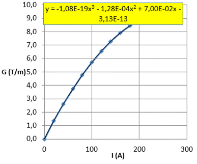
The following examples illustrate different possible configurations where the cavity is simulated using his 3D field map.
Example 1 (Absolute energy):
The cavity is tuned using a downstream TOF diagnostic (1) element later.
ERROR_CAV_NCPL_STAT 20 1 0. 0. 0. 0. 50 15 0
; Static RF errors are defined to 50% for amplitude and 15° for the phase
DRIFT 100 28 0
DRIFT 100 28 0
SET_SYNC_PHASE
TUNE_CAVITY 2010 75 25 1 0 0.1 0.1
FIELD_MAP 100 415.16 -45 28 1.83091 1.83091 0 0 spoke
DRIFT 100 28 0
; Position of the TOF1
DRIFT 100 28 0
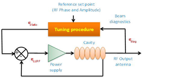
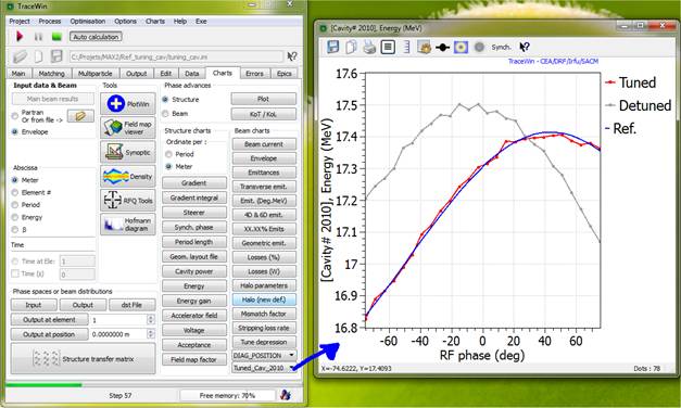
Before simulating cavity tuning, the static RF phase and amplitude errors defined in the error command will be considered when they are also selected in the "Error setup" box (see below), indicating which errors will be applied.
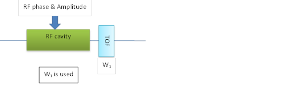
Using TraceWin output chart page, we can observe the cavity tuning procedure results. The gray curve (Detuned) show the initial RF tuning of the cavity which takes into account RF static error defined in this example (20% & 50°). The blue curve is the RF tuning objectives based on perfect model and the red one is the result of the cavity after the tuning procedure. Here, the procedure is based on a RF phase scan of ± 75° with 25 steps of measurement.
So, starting from the gray curve, the RF amplitude and phase are adjusted to minimize the difference between the results (red curve) with objectives (blue curve). This tuning is not perfect because diagnostics measurement errors are also included. In this example, a ±1% systematic error and a ±0.01% random noise are applied to the 26 beam energy measurements.
Example 2 (relative energy):
The cavity is tuned using a 2 x TOF diagnostics located upstream and downstream the tuned cavity, which corresponds to the measurement of the beam energy gain in the cavity.
ERROR_CAV_NCPL_STAT 20 1 0. 0. 0. 0. 50 15 0
; Static RF errors are defined to 50% for amplitude and 15° for the phase
DRIFT 100 28 0
; Position of the TOF1, 1 element backward
DRIFT 100 28 0
SET_SYNC_PHASE
TUNE_CAVITY 2010 75 25 -1 0 0.1 0.1 1 0 0.1 0.1
FIELD_MAP 100 415.16 -45 28 1.83091 1.83091 0 0 spoke
DRIFT 100 28 0
; Position of the TOF2, 1 element forward
DRIFT 100 28 0

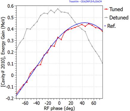
Example 3 (relative phase):
The cavity is tuned using the relative beam phase measurement. In this configuration, the distance between the cavity being adjusted and the BPM is an important parameter. We can see on the results curve, the effect of the 0.3 mm or BPM position and the 0.25° of measurement noise.
ERROR_CAV_NCPL_STAT 20 1 0. 0. 0. 0. 50 15 0
; Static RF errors are defined to 50% for amplitude and 15° for the phase
DRIFT 100 28 0
DRIFT 100 28 0
SET_SYNC_PHASE
TUNE_CAVITY 2010 75 25 1 1 0.1 0.1
FIELD_MAP 100 415.16 -45 28 1.83091 1.83091 0 0 spoke
DRIFT 100 28 0
; Position of the BPM, 1 element forward
DRIFT 100 28 0
![]()
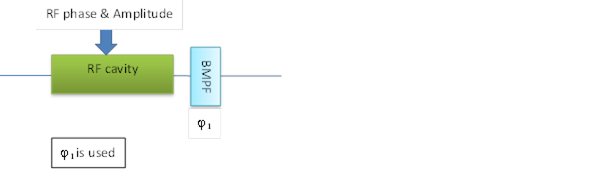

Example 4 (absolute phase):
The cavity is tuned using the absolute phase measurements of the beam according to master RF phase. In this configuration, a first measurement is done with RF cavity off.
DRIFT 100 28 0
DRIFT 100 28 0
SET_SYNC_PHASE
TUNE_CAVITY 2010 75 25 1 1 2.0 1.0 4 1 2.0 1.0
FIELD_MAP 100 415.16 -45 28 1.83091 1.83091 0 0 spoke
DRIFT 100 28 0
; Position of the BPM#1, 1 element forward
DRIFT 100 28 0
; This cavity is detuned during scan process
SET_SYNC_PHASE
FIELD_MAP 100 415.16 -44 28 1.83091 1.83091 0 0 spoke
DRIFT 100 28 0
; Position of the BPM#2, 1 element forward
DRIFT 100 28 0
![]()
![]()
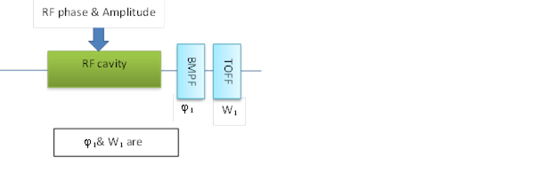
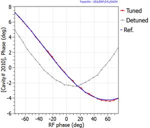
Example 5:
The cavity is tuned using the absolute phase and energy measurement of the beam.
DRIFT 100 28 0
DRIFT 100 28 0
SET_SYNC_PHASE
TUNE_CAVITY 2010 75 25 1 1 0.1 0.1 1 0 0.1 0.1
FIELD_MAP 100 415.16 -45 28 1.83091 1.83091 0 0 spoke
DRIFT 100 28 0
; Position of the BPM, 1 element backward
; Position of the TOFF, 1 element forward
DRIFT 100 28 0
![]()

|
|
|
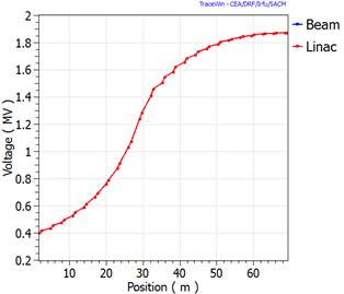
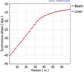
Example 6:
See “tuning_cav.ini” project in example list.
This example is the tuning results of a full linac composed of 45 cavities accelerating the beam from 17 MeV to 73 MeV. All cavities are tuned using only one beam phase monitor located about 1 meter downstream.
Without errors:
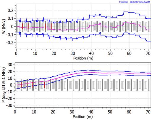
|
|
|


With errors:
The diagnostics position error is within ±0.3 mm and the phase measurement noise is within ±0.25°. To tune the cavity, the RF phase scan is within ±75° with 25 steps.
The initial RF errors are respectively set to 20% and 50° to simulate an initial tuning when operator doesn’t know at all the starting set point of the RF.
This result shown below corresponds only to one set of errors and statistics should be performed to be able to define accurately the acceptable error levels for this machine.
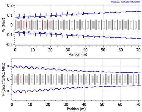
|
|
|
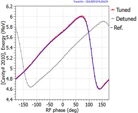
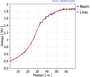
Despite huge initial errors, the final tuned cavity voltages and synchronous phases are close to the perfect machine. The output beam energy and phase differ from the reference ones, respectively by +0.04 MeV and -17 °. However the longitudinal acceleration and focalization give a very good transport (see below), envelope plots without beam centroid.
The consequence of using tuning procedure is to generate different longitudinal reference linacs. In other terms, there is an infinity of tuned machines. Another set of errors will give another linac tuning. Only statistical study is able to calculate the statistical behavior of the machine including cavities tuning considering errors applied to structure and diagnostics.
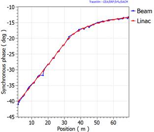
Remark: using 2 BPMs makes machine tuning much less sensitive to BPM position errors.
Example 7:
See “tuning_cav2.ini” project in example list.
This example is the tuning results of a full linac composed of 24 cavities accelerating the beam from 0.75 MeV to 40 MeV. All cavities are tuned using two beam phase monitors located in the following quadrupoles. Considering 1 mm of position errors, this scheme is very efficient.
Example 8 (DTL cavity):
Here, TOF is used to adjust RF field of a short DTL cavity. For long structure as DTL, the range of RF phase scan has to be large enough. To get realistical tuning simulation, DTL phases are set unsing absolute phase option (P) parameter of DTL_CEL = 3. The starting RF point errors are set using the coupling version of ERROR_CAV_XXX command.
; Proton @ 5.028 MeV
; Frequency = 352.2 MHz
ERROR_CAV_CPL_STAT 2000 1 0. 0. 0. 0. 20 120 0 0
SET_ADV 50
LATTICE 2 0
TUNE_CAVITY 2010 180 75 14 0 0.3 0.1
; 12 cells of DTL structure tank
DTL_CEL 88.0116 28 28 0.00502696 49 -49 66380.6 -50 10 3 0.103342 0.717258 -0.485156 -0.196227
DTL_CEL 88.3889 28 28 0.00833366 -50 50 69119.9 0 10 3 0.103784 0.723731 -0.475542 -0.198168
DTL_CEL 88.7837 28 28 0.0118928 49 -49 72056.6 0 10 3 0.104247 0.731513 -0.463853 -0.199942
DTL_CEL 89.1965 28 28 0.015516 -50 50 75048 0 10 3 0.104732 0.739058 -0.452425 -0.20129
DTL_CEL 89.627 28 28 0.0190039 49 -49 77950.8 0 10 3 0.105237 0.745 -0.443401 -0.202249
DTL_CEL 90.0759 28 28 0.0227398 -50 50 81051.7 0 10 3 0.105763 0.752113 -0.432503 -0.203008
DTL_CEL 90.5436 28 28 0.0265536 49 -49 84218.3 0 10 3 0.106312 0.759079 -0.421723 -0.203311
DTL_CEL 91.0306 28 28 0.0304112 -50 50 87435.5 0 10 3 0.106883 0.765757 -0.411327 -0.20332
DTL_CEL 91.5368 28 28 0.0343218 49 -49 90710.9 0 10 3 0.107477 0.772215 -0.401212 -0.20308
DTL_CEL 92.0622 28 28 0.0380767 -50 50 93904.6 0 10 3 0.108093 0.777295 -0.393249 -0.20285
DTL_CEL 92.6072 28 28 0.042087 49 -49 97300 0 10 3 0.108732 0.783367 -0.383636 -0.20219
DTL_CEL 93.1711 28 28 0.0457241 -50 50 100477 0 10 3 0.109394 0.787047 -0.377858 -0.201992
DRIFT 100 28 0
; Position of the TOF1
DRIFT 0 28 0
END

EoTL (V) is the maximum energy gain, φs (°) is the synchronous phase.
![]()
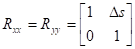
Where x’ being the horizontal beam centroid slope.
![]()
![]()
Δs (mm) is the drift length.
The non null 2´2 transfer sub-matrixes are:
![]() , and
, and ![]() .
.
fx, fy are focal length in meter
The non null 2´2 transfer sub-matrixes are:
![]() ,
, ![]() , and
, and ![]() .
.
θxy are the beam rotation XY angle in degre
The ellipsoid can be brought upright by rotations -θxy accomplished by applying the transfer matrixes:
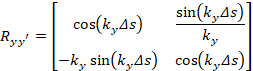 ,
,
The rotation is then applied:
![]() ,
,
Δs (mm) is the channle length, kx,y,z are focusing streength


Δs (mm) is the quadrupole length, G (T/m) its gradient.
For electrostatic quadrupole![]() , where Vo
is the voltage between electrode, βc beam speed and R is the
half distance between electrode.
, where Vo
is the voltage between electrode, βc beam speed and R is the
half distance between electrode.
Lets use ![]() , with
, with ![]() , the magnetic
rigidity of the particle.
, the magnetic
rigidity of the particle.
If q×G is positive, the quadrupole is focusing in the horizontal direction, else it’s defocusing.
The non null 2´2 transfer sub-matrixes are:
In the longitudinal direction, we have:![]() .
.
In the transverse direction, two possibilities:
![]() ,
, ![]() .
.
![]() ,
, ![]() .
.
EoTL (eV) is the maximum energy gain, φs (°) is the synchronous phase.
The reduced energy change in the gap is:
![]() ,
, ![]()
The phase shift in the gap is:
If βs = 0 : Δφ = 0 and Lscaled=L
else ![]()
![]()
The changes in the normalized momentum caused by the gap are given by:
![]() , With
, With ![]() and
and ![]() .
.
![]() .
.
The non null 2´2 transfer sub-matrixes are:
,![]() ,
, ![]() .
.
- If βs = 0 : ![]()
- If βs ¹ 0:
![]() ,
, ![]()
(* See Transit time factor definition according to βs
C: is a
coefficient allowing to keep the matrix determinant equal to: ![]()
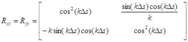
Δs (mm) is the solenoid length, B (T) its axis magnetic field.
Let’s use![]() , with
, with ![]() , the magnetic
rigidity of the particle.
, the magnetic
rigidity of the particle.
The non null 2´2 transfer sub-matrixes are:
![]() ,
,
![]() ,
,
![]() .
.
Δα (°) is the rotation angle, ρ (mm) is the curvature radius, n is the field index, ouv(mm) the aperture and HV means: horizontal (=0) or vertical bend (=1).
A positive bend (α>0) bends the particles to the right in the horizontal plane, regardless of the sign of the particle charge state. A negative α bends particles to the left.
![]() ,
, ![]() ,
, ![]() ,
, ![]() .
.
The non null 2´2 transfer sub-matrixes are:
![]() ,
,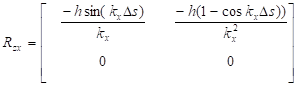 ,
,
![]() ,
,
![]() .
.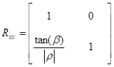
β (°) is the edge angle, ρ (mm) is the curvature radius in the bending magnet, g (mm) is the gap between the poles of the bending magnet, K1 and K2 are used in a development for the fringe-field correction. If they are equal to zero, K1 = 0.45 and K2 = 2.8. Set small values to cancel fringe-field correction.
ouv (mm) is the aperture and HV means: horizontal (=0) or vertical bend (=1).
The edge angle is treated as a thin lens. Ψ is the fringe-field correction.
![]() .
.
The non null 2´2 transfer sub-matrixes are:
![]() ,
, ![]() And
And ![]() .
.
![]() And
And ![]()
If Elec_flag equal 1
![]() and
and ![]()
Where x’ and y’ being respectively the horizontal and vertical beam centroid slope.
The dimension gc(mm) is
defined as: gap position ![]() .
.
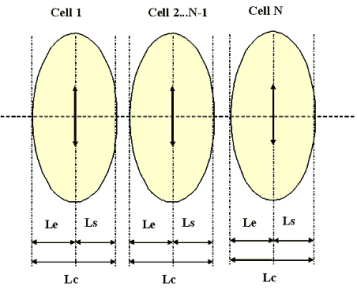
Cavity multi-gap (m, N, βg, EoT, θs, r, p, kEoTi, kEoTo, Dzi, Dzo, βs, Ts, kT’s,k²T”i, Ts, kT’i,k²T”i, To, kT’o,k²T”o)
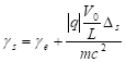
If m=0:
For cell1 : Le = ½ βλ +dzi, Ls = ½ βλ-dzi, Lc = βλ, EoT(1) = EoT (1+kEoTi.(Ti/Ts))
For cell2 to N-1 : Le = Ls = ½ βλ, Lc = βλ, EoT(2..N-1) = EoT
For cellN : Le = ½ βλ +dzo, Ls = ½ βλ - dzo, Lc = βλ, EoT(N) = EoT.(1+kEoTo.(To/Ts))
If m=1:
For cell1 : Le=1/4 βλ +dzi, Ls=1/4 βλ-dzi, Lc= ½ βλ, EoT(1)= EoT.(1+kEoTi.(Ti/Ts))
For cell2 to N-1: Le=Ls=1/4 βλ, Lc = ½ βλ, EoT(2..N-1)= EoT.(1+kEoTi.(Ti/Ts)
For cellN : Le=1/4 βλ+dzo,Ls=1/4 βλ - dzo, Lc= ½ βλ, EoT(N)= EoT.(1+kEoTo.(To/Ts))
If m=2:
For cell1 : Le=1/4 βλ+dzi + dzi, Ls=½ βλ-dzi, Lc= ¾ βλ, EoT(1)= EoT.(1+kEoTi.(Ti/Ts))
For cell2 to N-1: Le=Ls= ½ βλ, Lc = βλ, EoT(2..N-1)= EoT.(1+kEoTi.(Ti/Ts)
For cellN : Le=½ βλ +dz0, Ls=1/4 βλ - dzo, Lc= ¾ βλ, EoT(N)= EoT.(1+kEoTo.(To/Ts))
For all cases : EoTL= EoT(x.(Ls + Le))
Vo (V) is the voltage, Δs (mm) is the step length, L (mm) is the element length, and K (eV/mm²) is the transverse defocalisation contribution.
The reduced energy change in the gap is:
![]() .
.
Let’s use:
![]() and
and ![]() with
with ![]() and
and ![]() .
.
The non null 2´2 transfer sub-matrixes are:

![]()
|
|
Correction:
![]() have to be
validated
have to be
validated
L (mm) is the cavity length, N is the number of cells, EoT (eV/m) is the mean electric field of the cavity, θs (°) is the phase of the synchronous particle at the entrance of the cavity (relative to the R.F. phase.
Let's assume the electric field on the axis:
![]() ,
With
,
With ![]() .
.
The transverse electric field component can be deduced from Maxwell equations with a first order expansion:
![]() ,
,
Þ 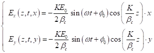
The same way, the transverse magnetic field component can be deduced:
![]() ,
,
Þ 
With ![]() ,
, ![]() , f the
R.F frequency and c the speed of light in vacuum.
, f the
R.F frequency and c the speed of light in vacuum.
Let's ps be the synchronous particle momentum at a given z, its evolution is given by:
![]() .
.
The particle momentum is: ![]() ,
,
With 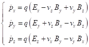
The evolution with time of the particle momentum p is given by:
![]() .
.
Let's δ be the momentum of the particle relative to that of the synchronous particle:
![]() .
.
We have: ![]() .
.
The evolution of δ is given by the equation:
![]() ,
,
![]() ,
,
![]() .
.
With ![]() ,
, ![]() and
and ![]() ,
,
We finally find at first order:
![]() .
.
Both focusing and damping effects can be observed.
Using: ![]() the matrix
transport can then be written over a small step dz:
the matrix
transport can then be written over a small step dz:
![]() ,
,
With: γs and γe being the synchronous normalized energy before and after the "gap",
![]() And
And
![]() .
.
The evolution of x' with time is driven by the equation:
![]()
![]() .
.
At first order, we finally have:
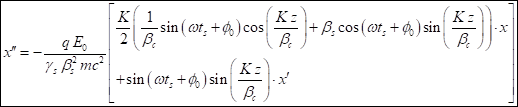 .
.
Both focusing and damping effects can be observed.
The matrix transport over a small step dz can then be written:
![]() ,
,
With: ![]() ,
,
And ![]() .
.
The differential equation can be written:
![]() ,
,
With: ![]()
And: ![]() ,
,
And: ![]() ,
,
The solution of this differential equation gives:
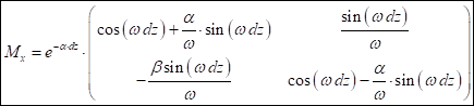 , If ω
is real,
, If ω
is real,
And
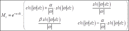 , If j ω
is real.
, If j ω
is real.
The Nc-cells cavity is divided
in n×Nc steps of length: ![]() .
.
As input, we have:
γo = γin; ![]() ;
; ![]() ;
; ![]() ,
, ![]() : Particle co-ordinates
at cavity input.
: Particle co-ordinates
at cavity input.
Then, we loop until reaching the end of the cavity:
For i from 0 to n×Nc-1 do
![]() ,
, ![]() ,
, ![]() ,
,
![]() ,
, ![]() ,
,
![]() ,
, ![]() ,
,
![]() ,
, ![]() .
.
L (mm) is the RFQ cell length, V(V) is the mean voltage of the cell, θs(°) is the phase of the synchronous particle, ro is the vane radius, m is the modulation, Tc is the transverse curvature and dP is a phase shift defined only dP which is a phase shift allowing to reset the output phases of Toutatis who does not own phase reference, Type parameter is defined bellow.
Cell type:
±2: Accelerating cell.
±3: Front-end cell.
±4: Transcell.
The sign of type being…..
![]() And
And ![]()
![]()
![]()
![]() , f the
R.F frequency and c the speed of light in vacuum.
, f the
R.F frequency and c the speed of light in vacuum.
The matrix transport can then be written over a small step dz:
![]() ,
,
With: γs and γe being the synchronous normalized energy before and after the "gap",
![]()
![]()
C3 depend of the cell type.
±2 or ±3: ![]()
±4: ![]()
The matrix transport over a small step dz can then be written:
![]() ,
,
![]()
With: ![]() ,
,
![]()
And ![]() .
.
![]() And
And ![]()
C1 , C2 and S depend of the cell type.
±2: ![]() ,
,![]() ,
, ![]()
+3: ![]() ,
,![]() ,
,
![]()
-3: ![]() ,
, ![]() ,
, ![]()
+4: ![]() ,
,![]() ,
, ![]()
-4: ![]() ,
,![]() ,
, ![]()
With type[n+1] being the type from the next cell and type[n-1] the type from preceding cell.
The rfq cell is divided in ×N steps of length: ![]() .
.
As input, we have:
γo = γin; ![]() ;
; ![]() ;
; ![]() ,
, ![]() : Particle
co-ordinates at cavity input.
: Particle
co-ordinates at cavity input.
Then, we loop until reaching the end of the cavity:
For i from 0 to N-1 do
![]() ,
, ![]() ,
, ![]() ,
,
![]() ,
, ![]() ,
,
![]() ,
, ![]() ,
,
![]() ,
, ![]() .
.
The following paper come from a CEA report named:
“Transfer matrix of a constant gradient alpha magnet for ELSA extension”
Ref: DSM/DAPNIA/SACM/2002/13
N. Pichoff
In this paper, the motion equation of a particle in such a device is linearised to get the transfer matrix. The matrix has been validated with a step-by-step integration of the motion of a particle in the magnetic field.
The trajectory of the synchronous particle (ideal trajectory is, by definition, in the plan (X, Y)). The frame origin is the point where the particle enters the magnet. The X direction is the direction of the magnetic field gradient. At any position, the main trajectory makes an angle θs with the X axis. The entrance angle for negative particle θse is: -40.71°. With this particular angle, the synchronous particle exits the magnet at the same position as the entering particle (and with the opposite angle).

In this frame, the magnetic field is:
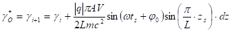
The synchronous particle with particle charge q state moves in the (X, Y) plan.
Its motion equations with time t are:

p is the particle momentum, v its velocity,
giving:

![]() is the particle
momentum modulus,
is the particle
momentum modulus,
s is the
curvilign abscissa, with ![]() .
.
These equations have to be solved using as initial conditions:
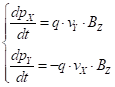
The maximum penetration of the particle XM in the magnet can be calculated the following way:
![]() Þ
Þ ![]() .
.
At maximum penetration, one has:![]() , giving:
, giving:
![]() .
.
The length L of the trajectory is obtained from the integration of:
![]() .
.
One obtains:
![]() .
.
This integral cannot be solved analytically but can be easily calculated numerically.
In the transfer matrix formalism, a beam particle is referenced, at a given curvilign abscissa s, to the synchronous particle in a 6D phase-space, with a 6-coordinates vector:
 ,
,
with:
- x is the particle transverse position in the deviation plan,
- x’ is the particle
transverse slope in the x direction. ![]() ,
,
px the x-component of the particle momentum, and ps the s-component of the particle momentum,
- y is the particle transverse position orthogonal to the x direction,
- y’ is the particle
transverse slope in the y direction. ![]() ,
,
py the y-component of the particle momentum,
- φ is the time difference between the particle arriving in s (t) and the synchronous particle arriving in s (t(S)). This time is normalized with the RF frequency fRF.
![]() ,
,
- δ is the particle momentum p relative to the synchronous particle momentum p(S).
![]() .
.
In the matrix formalism, the particle vector change from a point (1) to a point (2) is given by:
![]() ,
,
where [T] is the transfer matrix from (1) to (2). The coefficients of [T] are:
![]() .
.
i is the line index, j is the column index (between 1 and 6).
The matrix coefficients can be calculated by varying the input particle coordinate along each direction independently and looking at the output coordinates.
Matrix third and fourth columns
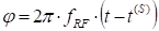
Calculus of T1,1
D is at the intersection of (O), C and the circle with centre E and radius ρ. Its coordinates satisfy:
![]() .
.
Giving: ![]() ,
,
with: ![]() .
.
As: ![]() , one
has:
, one
has: ![]() .
.
The solution of (X) is obtained giving a reduced discriminator:
![]() ,
,
giving:
![]() .
.
A first order development in ![]() and
and ![]() gives:
gives:
![]() .
.
This gives the coordinates if D:
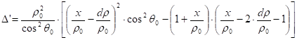
The final position of the particle in the moving frame is then:
![]()
Calculus of T2,1
![]() ,
,
with: ![]() .
.
At first order, one has:
![]() ,
,
giving :
![]()
Calculus of T5,1
![]() .
.
with: ![]() .
.
One obtains finally:
![]() .
.
The other terms (T3,1, T4,1 ,T6,1) are equal to zero.
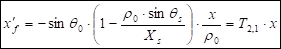
Calculus of T1,2
D is at the intersection of (O), C and the circle with centre E and radius ρ. Its coordinates satisfy:
![]() .
.
Giving:
![]() .
.
The solution of (X) is obtained giving a reduced discriminator:
![]() .
.
A first order development in ![]() gives:
gives:
![]()
This gives the coordinates of D:
![]()
The final position of the particle in the moving frame is then:
![]()
Calculus of T2,2
![]()
with: ![]() .
.
At first order, one has:
![]() ,
,
giving :
![]()
Calculus of T5,2
![]() .
.
with : ![]() ,
,
as: ![]() ,
,
one has: ![]() .
.
One obtains finally:
![]() .
.
The other terms (T3,2, T4,2 ,T6,2) are equal to zero.

Calculus of T1,6
D is at the intersection of (O), C and the circle with center E and radius ρ. Its coordinates satisfy:
![]() .
.
Giving:
![]()
with: ![]() .
.
As: ![]() , one
has:
, one
has: ![]() .
.
The solution of (X) is obtained giving a reduced discriminator:
![]() .
.
A first order development in ![]() gives:
gives:
![]()
This gives the coordinates of D:
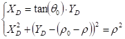
The final position of the particle in the moving frame is then:
![]()
Calcul of T2,6
![]()
With: ![]() .
.
At first order, one has:
![]() ,
,
Giving:
![]()
Calcul of T5,6
![]() .
.
with: ![]() ,
,
One obtains finally:
![]() .
.
The terms (T3,6, T4,6) are equal to zero, the term T6,6 is equal to 1.
The output position, slope, energy do not depend on the input phase φ:
The terms (T1,5, T2,5, T3,5, T4,5, T6,5) are equal to zero, the term T5,5 is equal to 1.
The equation of motion along Z direction is:
![]() .
.
For the matrix calculation, one uses a first order development of the force, giving:
![]() .
.
This equation is the classical one in a
quadrupole with gradient: ![]() .
.
The associated matrix coefficients are:
![]() ,
,
![]() ,
,
![]() ,
,
With: ![]() .
.
The other coefficients are equal to 0.
The final matrix of a fraction of a alpha magnet (on which, Xs and θs are kept almost constant) :

With: ![]() ,
,
And: ![]() .
.
The matrix of the full element is a product of all matrixes for varying Xs and θs.
Definition of matched beam
Mismatch factor
Twiss parameters and acceleration
Beta function definition
Dispersion definition
Synchronous phase definitions
Particle motion in electromagnetic field
3D field development for a quadrupole
Core–Halo evolutions along the accelerator
Stripping losses
x, y, z is in a direct frame.
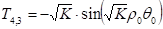
![]() ,
, ![]() ,
, ![]()
![]()
![]()
![]()
![]()
v, and b are the particle velocity and reduced velocity,
mc2, E, W and g are the particle rest mass energy, total energy, kinetic energy and reduced energy,
p and gb are the particle momentum and reduced momentum.
c is the physical maximum velocity (speed of light in vacuum).
λ and f are respectively the free-space wavelength and the RF frequency of an electromagnetic field.
In an accelerator, the transport of the beam particles is generally described as a function of the abscissa s, on a reference trajectory followed by a reference particle.
Each particle is represented by a 6 coordinate vector whose 3 coordinates represent the position and 3 represent the motion of the particle in the real space.
Where ![]() is a vector
representing the particle position in the phase-space:
is a vector
representing the particle position in the phase-space:  ,
,
In linear forces, the phase-space coordinates of a particle at location s2 can be deduced from those at the location s1 along an accelerator, by a single matrix multiplication:
![]() ,
,
x, y and z being respectively the horizontal, vertical and longitudinal position of the particle in the bunch (relative to a synchronous particle. ps is the synchronous particle momentum, and δ=(p‑ps)/ps, with p being the particle momentum.
R is the 6´6 transfer matrix between s1 and s2. In TraceWin this matrix is partitioned into 2x2 matrices to simplify and accelerate the calculations.
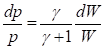 .
.
In order to be able to use this formalism,
the space charge force is considered
as linear. To calculate the space-charge effect, the real beam is replaced by
an equivalent uniform beam having identical rms properties (sizes and
emittances. The total emittance of the equivalent uniform bunched beam in each
phase plane is then 5 times the rms emittance, and its envelope size is ![]() times its rms
size. For a continuous beam these factors are 4 for the emittance and 2(
times its rms
size. For a continuous beam these factors are 4 for the emittance and 2(![]() for envelope.
for envelope.
Lets define
![]() as the mean value
of the w particle property over the beam at location s.
as the mean value
of the w particle property over the beam at location s.
The beam phase-space position is defined by:
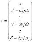
The beam rms sizes are defined by: ![]() , with w used for
x, x', y, y', z or δ .
, with w used for
x, x', y, y', z or δ .
The beam rms correlation: ![]() , with w and v
used for x, x', y, y', z or δ.
, with w and v
used for x, x', y, y', z or δ.
The beam rms unnormalized emittances: ![]() with w used for
x, y and z.
with w used for
x, y and z.
Note: In the preceding definition, z'
is defined as ![]() , vz and vzδ being
the longitudinal velocities of respectively the particle and the synchronous
particle. Most of the time, δ is used rather than z'. In
that last case, the emittance is defined by the conversion from εz
to εzδ.
, vz and vzδ being
the longitudinal velocities of respectively the particle and the synchronous
particle. Most of the time, δ is used rather than z'. In
that last case, the emittance is defined by the conversion from εz
to εzδ.
In case of linear forces, the beam can be
represented in sub phase planes by ellipses whose equation can be written: ![]() , where :
, where :
ew is the unnormalized beam effective emittance (which is the full emittance of a homogenous beam define as 5 times the rms-emittance for bunched beam and 4 times that of a continuous beam).
![]() ,
, ![]() , and
, and ![]() are the beam
Twiss parameters satisfying the relationship:
are the beam
Twiss parameters satisfying the relationship: ![]() .
.
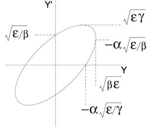
The beam can be represented by a matrix, called the σ-matrix defined as:
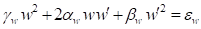 .
.
The evolution of the σ -matrix along the line from s1 to s2 can be calculated with the transfer matrix R:
![]() ,
,
Where RT is the transpose of R and [σ] is the beam σ-matrix. Like with the transfer matrixes the σ‑matrixes can be partitioned into 2x2 matrices:
![]() .
.
The elements are divided into small steps, whose transfer matrixes are used to transport the beam σ-matrix. The space-charge effect is applied at each step.
The 2x2 extracted σ-matrix can be written in terms of Twiss parameters.
![]() .
.
We observe that ![]()
Let's R be the transfer matrix of a
lattice of a periodic structure: 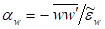 .
.
The 2x2 extracted diagonal matrix can be written:
![]() ,
,
Where αwo, βwo, and γwo are the Twiss parameters of the beam matched to the lattice, and σwo is the zero-current phase advance per lattice in the [w-w’] phase plane.
The mismatch factor (as defined above between the two ellipses)
![]()
and
![]()
is given by
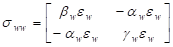
Where
![]()
For periodic structure, the chart “mismatch factor” form “Charts” tab-sheet compare for each period the input and ouput Twiss parameters.
In case of acceleration, the determinant of the transfer matrix is not equal to 1, and the matrix cannot be written with the Twiss parameters, as defined before. To extract the Twiss parameters of the matched beam from the transfer matrix when there is acceleration, we use the matrix defined as below:
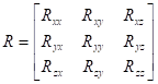 ,
,
Where βi and γi are the relativistic parameters at the input and βo and γo are the relativistic parameters at the output of the lattice. Now, the R' matrix determinant equals 1.
The Twiss parameters of the matched beam under acceleration conditions can then be deduced from the R' matrix:
![]() ,
, ![]() ,
, ![]() ,
,
![]() ,
, ![]() ,
, ![]() ,
,
![]() ,
, ![]() ,
, ![]() ,
,
![]() ,
, ![]() ,
, ![]() ,
,
Where, r’ij is a R' matrix coefficient (ith row, jth column and αwo, βwo, and γwo are output Twiss parameters of the matched beam in the [w-w’] phase plane).
β and γ being the beam reduced velocity and energy, λ the RF wavelength in vacuum, mc² the particle rest energy, we have in the paraxial approximation conditions the following relationship between parameters:
![]() ,
,
But if the beam shows a divergence this relation becomes:
![]()
Δφ and z being the RF phase and the position of a beam particle relative to the synchronous one.
![]() ,
,
In the general case with a synchronous particle and a generator particle these relation become:
![]()
![]()
ΔW, z' and δ being the energy, velocity and momentum of a beam particle relative to the synchronous one.
![]() ,
,
εw and εzn being the normalized longitudinal emittances, εz and εzδ being the unnormalized longitudinal emittances of the beam in respectively the [z-z'] and the [z- δ] phase planes.
![]() ,
,
βw, βz and βzδ are the β-Twiss parameters of the beam in respectively the [Δφ-ΔW], [z-z'] and [z-δ] phase planes.
![]() ,
,
αw, αz and αzδ are the α-Twiss parameters of the beam in respectively the [Δφ-ΔW], [z-z'] and [z-δ] phase planes.
![]() ,
,
γw, γ z and γzδ are the γ-Twiss parameters of the beam in respectively the [Δφ-ΔW], [z-z'] and [z-δ] phase planes.
Longitudinal normalization is defined so that the normalized, emittance is independent of the chosen longitudinal coordinate, (Z', dp/p or ΔW).
![]()
![]()
![]()
![]()
(n = Normalized,
![]() =
= ![]() )
)
![]() n
n
![]()
![]()
![]()
![]()
Imporvement proposed by Molodozhentsev Alexander, 2016 for very specific case like laser-driven election accelerators, acoording to the following publication:
“Intrinsic normalized emittance growth in laser-driven electron accelerators, M. Migliorati et al.”
https://journals.aps.org/prab/abstract/10.1103/PhysRevSTAB.16.011302
Normaliszed transverse emittance for ultra relativistic electron beam is coorected according to formul below:
![]()
This correction could be activated by selecting “Emittance correction” option from box “Simulation options” in “Main’ tab-sheet.
The βxx’ and βyy’ function plotted in envelope charts are defined as following:
![]() and
and ![]()
s, the beam matrix and T, the transfer matrix and e is the normalized emittance at the beginning of the structure and bg is the reduced momentum at considered position.
The H disp and V disp function plotted in envelope charts are defined as following according to selected option:
The defaut dispersions are defined like following:
Hor_Disp = T16 / T66
Ver_Disp = T36 / T66
If option « Use default dispersion def. » from « Main » tab-sheet is not choosen then:
Hor_Disp = T16
Ver_Disp = T36
T is the transfer matrix.
In tracking way, dispersions are defined like following:
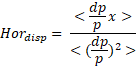

The energy gain of a particle in a cavity is given by:
![]()
Its depends on the cavity field amplitude ![]() and RF phase seen
by the particle
and RF phase seen
by the particle ![]() when it is at
position
when it is at
position ![]() . This RF phase is
given by equation:
. This RF phase is
given by equation:
![]()
Where:
-
![]() is the RF phase when particle enters the cavity at position
is the RF phase when particle enters the cavity at position ![]() . For a given
particle, it varies linearly (of slope 1 with respect to the phase of the RF
field in the cavity).
. For a given
particle, it varies linearly (of slope 1 with respect to the phase of the RF
field in the cavity).
- ![]() is the particle
reduced velocity at position
is the particle
reduced velocity at position ![]() ,
,
-
![]() is the wavelenght
of the RF field in the cavity.
is the wavelenght
of the RF field in the cavity.
In TraceWIN, the beam dynamics in a cavity
is numerically integrated in the field map starting at ![]() .
.
Nevertheless, most of the accelerator physicists are used to designing linacs with cavities operating at a given:
- “effective voltage”, ![]() and
and
-
“synchronous phase”, ![]() .
.
as parameters of a simplified model of the energy gain in the cavity []:
![]()
This means that a “common language” has to be established in order to translate these parameters in real amplitude and phase of a field map.
TraceWIN proposed 2 models to define the effective voltage and the synchronous phase explained below.
NB1: The user can chose one or the other model, remembering that the beam dynamics is finally calculated in the field map whatever his choice. Nevertheless, the chosen model has an impact on the way the cavity is tuned for given effective voltage and synchronous phase.
NB2: The two models gives the same effective voltage and synchronous phase when the field is low (the velocity change is negligible in the cavity)
NB3: Both
models give 0 energy gain for ![]() but only model 2 gives maximum energy gain for
but only model 2 gives maximum energy gain for ![]() .
.
NB4: The phase acceptance associated to a given synchronous phase depends on the chosen model and the acceleration conditions. It is recommended to check it with multiparticle simulations.
Historic model:
Starting from the exact calculation of energy gain:
![]()
Adding and subtracting an arbitrary phase ![]() in the cosine:
in the cosine:
![]()
Using trigonometric laws: ![]() , one gets:
, one gets:
![]()
![]()
This energy gain can then be “naturally” modelled by:
![]() ,
,
by choosing ![]() cancelling the second term, i.e.:
cancelling the second term, i.e.:
![]()
Using trigonometric laws: ![]() , one gets:
, one gets:
![]()
Leading to a definition of the synchronous
phase ![]() :
:
![]()
and of the effective voltage:
![]()
PS: one notes that, in these conditions:
![]()
New model:
New model proposed by Jean-Michel LAGNIEL (GANIL).
See « Longitudinal beam dynamics at high accelerating fields, what changes ? », ROSCOFF 2021.
Equalizing the real energy gain of the synchronous particle with the one given by the model:
![]()
![]()
![]()
![]() is calculated
numerically from the field map.
is calculated
numerically from the field map.
Equalizing the variation with RF phase of the real energy gain with the variation with synchronous phase of the modelled energy gain around the synchronous particle (linearization):
![]()
![]()
![]()
![]() is calculated
numerically from the field map.
is calculated
numerically from the field map.
Leading to a definition of the synchronous
phase ![]() :
:
![]()
and of the effective voltage:
![]()
These following definitions are used in all accelerating element.
T: is the usual time factor transit given by SUPERFISH.
T’: is the T’ from SUPERFISH time -2π
T”: is the T” from SUPERFISH time -4 π²
![]() ,
,
![]() … With
… With
![]() .
.
The electric field is corrected according to T(β).
Coordinate transformations are given in Wangler's book page 202:
TraceWin calculates the particle phase advance in two ways. The first one is the extraction of the phase advance from the transfer matrix of the lattice (k0x,y, μ or σo). The second one is done by the beta function integration along a lattice giving the phase advance with (σ or without σo space charge):
![]() with L is the
lattice length and
with L is the
lattice length and ![]() .
.
x is the beam RMS or effective size and εx the unnormalized RMS or effective emittance.
with 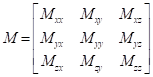 the transfer matrix of the lattice
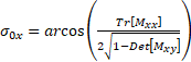 ,
, 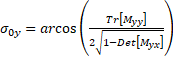 and
and ![]() with
with ![]()
The first phase advance type can be plotted from the “Phase advance”->”Structure”.of “Chart” page And the second one can be plotted from the “Phase advance”->”Beam” of “Chart” page
Use in the error studies in order to know the beam gravity evolution, It’s defined like below:
![]()
![]()
![]()
![]()
![]()
![]()
x & y are the beam gravity position and N is the number of run or linac.
In a one dimension linear motion (described in (pi, qi) phase-space, the following quantities are kinematic invariants):
![]()
![]()
< > is the average value over the beam distribution.
One defines the halo parameter, Hi (i for x, y, or z direction, as a ratio between a function of the fourth order momentum and the second order momentum):
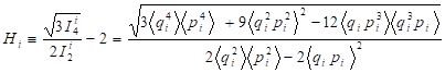
This quantity is conserved in linear forces and by homothetic transformation of the beam distribution.
It is normalized and centered in order to have:
- Hi = 0, for uniform elliptical distribution,
- Hi = 1, for Gaussian elliptical distribution.
From ref: “PHYSICAL REVIEW SPECIAL TOPICS - ACCELERATORS AND BEAMS,VOLUME 5, 124202 (2002)“, “Beam halo definitions based upon moments of the particle distribution (C. K. Allen and T. P.Wangler) “
In TraceWin the gradient definition is defined as following:
![]()
Where:
n = 2 Quadrupole
n = 3 Sextupole
n = 4 Octupole
With: B0, the magnetic field (T on the pole and a, the half aperture).
This definition depends of computer programs:
![]()
Magnetic stripping
H- beam passing through strong magnetic field causes beam losses. They can be visualized in multiparticle tracking mode when the option is choosen (“Magnetic stripping” from “Multiparticle” tab-sheet). A specific file is created to store them during simulation, see: Magnetic stripping file
Gaz stripping
H- beam passing through gaz causes beam losses. They can be visualized in multiparticle tracking mode when the option is choosen (“Gas stripping” from “Multiparticle” tab-sheet). A specific file is created to store them during simulation, see: Gas stripping file
The different cross-sections of the gases present must be specified in the structure file (*.dat), with the command Gas pressure
Intra-beam stripping
An analytical estimate of the beam losses due to the intrabeam particle collisions resulting in stripping of H- ions is available using “Intra-beam strip.” button from “Charts” tab-sheet. The equation used below is taken from the following publication: https://arxiv.org/ftp/arxiv/papers/1207/1207.5492.pdf
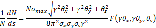
![]()
N is the number of particle in the bunch
σmax = = 3.6.10-15 cm2 is an approximation of the electron stripping cross-section if the velocity spread is inside of the cross-section plateau (see figure1) of the publication.
γ is the relativistic factor
σx,y are the transverse rms bunch sizes
ss and qs are the rms bunch length and the relative rms momentum spread
This estimation is available ethier in envelope mode or in multipaticle mode.
In the envelop simulation, the space-charge (SC force is linearized assuming an equivalent uniform beam if the beam is respectively continuous or bunched). The number of SC kicks is given by the parameter “Step of calculation per βλ” in the “main” sheet.
In a free space, the motion equation of a particle, feeling only space-charge force, can be written along one direction in the beam frame R*:
![]() ,
,
![]() being the w component of the space-charge force (divided by
the particle rest mass).
being the w component of the space-charge force (divided by
the particle rest mass).
All the quantities with a star (* are expressed in the beam frame R*), all quantities without star are expressed in the laboratory frame R.
We have, from the Lorentz transform:
![]() ,
, ![]() ,
, ![]() ,
, ![]() ,
,
and:
![]() .
.
The derivation with s, the beam longitudinal position used as independent variable, gives:
![]() .
.
In the longitudinal direction, one has:
![]() .
.
Continuous beam
In continuous beam, no space-charge force acts along the longitudinal direction, and:
![]() ,
, ![]() ,
,
with: ![]() , the beam
generalized perveance.
, the beam
generalized perveance.
ax, ay, are the semi-axes of the homogeneous ellipse (2 times the rms beam sizes), I is the average beam current, ε0 is the vacuum permittivity.
Bunched beam
The space-charge force w-component (w) for x, y or acting on the particles:
![]() ,
,
with: ![]() ),
),
and ![]() is the form
factor such as:
is the form
factor such as:
![]() .
.
![]() ,
, ![]() and
and ![]() are the beam semi-axes of a uniform ellipsoid (Ö5) times the rms
beam sizes in the beam frame, Q is the bunch charge, εo is the vacuum
permittivity. Note that:
are the beam semi-axes of a uniform ellipsoid (Ö5) times the rms
beam sizes in the beam frame, Q is the bunch charge, εo is the vacuum
permittivity. Note that: ![]() .
.
The form factor integral calculation
depends on the ratios ![]() and
and![]() . If they are
lower than 12 the integral is calculated by the Gauss method with a very good
precision. If they are greater than 12 (which happens obviously when the beam
is ultra-relativistic due to the Lorentz transformation an expended development
is used and slightly reducing the result precision).
. If they are
lower than 12 the integral is calculated by the Gauss method with a very good
precision. If they are greater than 12 (which happens obviously when the beam
is ultra-relativistic due to the Lorentz transformation an expended development
is used and slightly reducing the result precision).
Space-charge application
Frame change
The space charge impulse should be applied in the beam frame. Before any application, the beam σ-matrix should be written from the laboratory frame to the beam frame by making the transformation:
![]() ,
,
with: 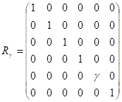 .
.
After the application of space-charge impulse (taking into account the beam coupling, the σ-matrix should be written back to the laboratory frame):
![]() ,
,
with: 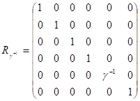 .
.
Beam coupling or tilted.
Due to the elements (magnetic coil or dipole or initial conditions), the beam ellipsoid in [x-y-z] space can be tilted. In this case, the beam ellipsoid (in the beam frame must first be transformed to a coordinate system in which it is upright before applying the space-charge impulses).
If the ellipsoid is tilted in the [x-y] plane, the angle between the x-axis and the axis of the elliptical projection on the [x-y] plane is:
![]() ,
,
with σ ij , σ -matrix elements.
If the ellipsoid is tilted in the [x-z ] plane:
![]() .
.
If the ellipsoid is tilted in the [y-z] plane:
![]() .
.
The ellipsoid can be brought upright by rotations of angles –θxy (or -θxz and -θyz accomplished by applying the transfer matrixes):
,
Rxz and Ryz can be obtained the same way.
The rotation is then applied:
![]() ,
,
![]() .
.
When the ellipse is upright, the space-charge impulses can be applied. The three reverse rotations can then be applied:
![]() ,
,
![]() .
.
Space-charge impulse
The space-charge kick applied on distance Δs (the calculation step uses the transfer matrix Rce):
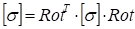 .
.
The space-charge impulse is applied in the bunch frame, where the beam ellipse is upright:
![]() .
.
Finally, the total space charge effect is given by:
![]() .
.
In the Partran simulation, the user can select its space-charge routine in the “Multiparticle / Partran space charge options” sheet.
- PICNIR (2D – (r, z), Particles In Cells Numerical Integration between Rings, is based on the SCHEFF model. It considers a beam with a transverse circular symmetry. If it is not the case, a correction is applied which is less and less adequate as much as the beam is not circular. The first parameter gives the total number of lattices in radial ® direction, the second gives the total number of lattices in longitudinal (z) direction. The mesh size is adjusted from 0 to 3.5 times r-rms in transverse, and to +/- 3.5 times z-rms in the longitudinal. The space-charge force outside the mesh is this of an equivalent gaussian beam.
Set number of lattice, Nz, lower than 0 allows to cancel to longitudinal forces.
- PICNIC (3D) – (xy, z), Particles In Cells Numerical Integration between Cubes, is a fully 3D space-charge routine. The first parameter gives the half-number of lattices in horizontal (x)) and vertical (y directions, the second gives the half-number of lattices in longitudinal (z direction. Its options are :
o Weight: if 0, the particle charge is deposited in the lattice where it stands. If 1, the particle charge is distributed in the closest lattices (small smoothing). The nominal value is 0.
o Mesh/rms: the mesh full size is adjusted around the beam to +/- Mesh/rms time rms sizes (x, y and z. The nominal value (if one sets 0 is 3.5). The space-charge force outside the mesh is this of an equivalent gaussian beam.
o Skip: in order to slightly speed-up the space charge calculation, one can depose every Nth particle in the mesh. This parameter is N. The nominal value is 1.
- Special: written for dedicated user.
- CE_CYL: written for dedicated user.
- My space-charge: space charge routine defined from external library. See example shown in following chapter.
The number of SC kicks in field maps or in DRIFT is set in the “Multiparticle / Partran step of calcul” sheet. For all hard-edge elements (SOLENOID, BEND…), the SC kick is applied at its middle. If you want increase the SC kick rate, please cut the element in many pieces.
For DTL cell, QUAD & QUAD_ELE elements, multi SC kick can also be applied according to proposed options selected.
In all cases, the procedure is the following:
- the bunch, whose distribution is given at a given abscissa, is extended to the time of the CoG in bunch frame (where the average velocity is zero),
- the mesh size is calculated from the bunch RMS sizes,
- the only electric field is calculated in the bunch frame.
- the SC kicks are applied to the particles momentum in the bunch frame,
- the particles new angles and energy in laboratory frame are deduced.
The change of frames used Lorentz transformation. In case of ultra-relativist bunches in which particles can be relativistic even in bunch frame, the SC routine reaches one of its limits.
When the bunch is not short compared to the intra-bunches distance, effect of neighbor bunches are taken into account and particles out of +/- 180° are temporary “moved” into the bunch (with 360° jumps by the SC routine to estimate their contribution to the SC and calculate the SC they fill).
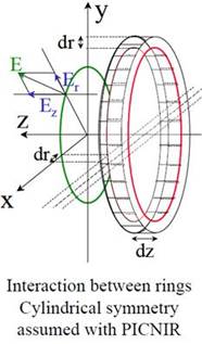
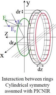
Recommendations for user:
- Have a look on https://accelconf.web.cern.ch/l98/PAPERS/MO4042.PDF to understand some subtleties of SC routines.
- PICNIR should be used with almost circular beams or to accelerate the calculus but to the expense or a lower accuracy.
- Use lattices with aspect ratio (in bunch frame as close as 1 as possible).
Adjust the number of SC lattices with the number of particles. For example, in PICNIC, we recommend to use 7×7 cells on ±3.5s mesh with 10k particles to tune a linac, 10×10 cells on ±4s mesh with 100k particles to finalize the linac design and 15×15 cells on ±5s with 1M particles to explore the tails and >10M particles for outside communication (in that case, choose the mesh size you want !)
Have a look on noise anaylisis: Phys. Rev. ST Accel. Beams 17, 124201 (2014)
This feature allows to each user to develop its own space-charge routine. A detailed example following explains how to perform it. Use the following ‘main.cpp’ file and compile it as a dynamic library. This library has be located either in the structure (*.dat directory or in the executable directory).
/***************************************************************************
main.cpp
Windows -> Dynamic library (dll
Linux or MacOS -> Dynamic shared object (so, dylib
-------------------
begin : Wed Dec 1 2010
copyright : (C 2010 by URIOT Didier
email : duriot@cea.fr
***************************************************************************/
#ifdef _WIN32
#include <windows.h>
#define DLL_EXPORT __declspec(dllexport)
#else
#define DLL_EXPORT
#endif
#include <cmath>
#include <cstdio>
#include <cstdlib>
#include <cstring>
#ifdef __cplusplus
extern "C" {
#endif
//--------------------------------------------------------------------
//-- MY_SC - MY_SC - MY_SC - MY_SC - MY_SC - MY_SC - MY_SC -----------
//--------------------------------------------------------------------
//
// You have to compile your space-charge routine as an dll
// - my_space_charge.dll (for windows)
// - my_space_charge.so (for linux)
// - my_space_charge.dylib (for MacOS)
//
// Commands to compil and link GNU gcc compiler in Windows:
// g++.exe –m32 -Wall -c main.cpp -o main.o
// g++.exe –m32 -shared -Wl,--dll main.o -o my_space_charge.dll
// If you use 64bits TraceWin version replace both -m32 by -m64
// Commands to compil and link GNU gcc compiler in MAC OS:
// g++ -m32 -Wall -pedantic -c main.c -o main.o
// g++ -m32 -Wall -shared -dynamiclib main.o -o my_space_charge.dylib
// If you use 64bits TraceWin version replace both -m32 by -m64
// MY_SC syntax example
// repect the name of the routine
int DLL_EXPORT space_charge(double Zs, double ds,int mesh1,int mesh2,int Nele,int npart,double *cord,double *loss,double freq,double mass0,int q,double *ws,double *Ibeam,double *extra_param,char *error_mess)
{
// Zs : Current position in the element (from ds/2 to Length-ds/2 (m))
// ds : kick applied distance (m)
// mesh1 : First parameter of the SC option in sheet “multiparticle” sheet
// mesh2 : Second parameter of the SC option in sheet “multiparticle” sheet
// cord : See example (drift)
// loss : see example (drift)
// freq : beam frequency (Hz)
// mass : Particle mass (eV)
// q : particle charge state
// *ws : reference kinetic energy (eV (can be modified))
// *Ibeam : Beam current (A (can be modified)
// *extra_param : Not used
// error_mess : TraceWin stop and show this error message if this function return 0
// if error_mess!="" and function return 1, this message is print to the standard console without stop TraceWin
double zzs,bgs,gams,betas;
double x,y,xp,yp,z,dpsp,w,gamma;
strcpy(error_mess,"");
zzs=(*ws/mass0);
bgs=sqrt(zzs*(2.+zzs));
gams=1.0+zzs;
betas=bgs/gams;
// drift treansport example, has to be replace by your SC routine
for (int i=0;i<npart;i++) {
if ((int)loss[i]==0) {
x=cord[i*6]; // m
xp=cord[i*6+1]; // rad
y=cord[i*6+2]; // m
yp=cord[i*6+3]; // rad
z=cord[i*6+4]; // m
dpsp=cord[i*6+5]; // dp/p
x=x+ds*xp;
y=y+ds*yp;
w=dpsp*betas*betas*gams*mass0+(*ws);
gamma = 1+w/mass0;
z=z+dpsp*ds/(gamma*gamma);
cord[i*6]=x;
cord[i*6+2]=y;
cord[i*6+4]=z;
}
}
return(1;
}
#ifdef __cplusplus
}
#endif
The equations of particle motions in electromagnetic field (RF) or static defined below are mainly uses in FIED_MAP elements for each particle (Partran) and for beam centroid (Envelope) with linearization.
The variation of the amount of movement of a particle with charge q and mass m is within an electromagnetic field:
![]()
In Cartesian coordinates:

With:
![]() et
et ![]()
Then:
![]()
Finally, we get:
![]()
![]()
As regards the longitudinal dynamics, the variables used are generally either kinetic energy T, or the amount of movement of the particle p. The variation of these parameters is derived from the relationship:
![]() .
.
Given:
![]()
![]()
Then:
![]()
And:
![]()
In the PIC code, these equations must be integrated step by step
Under the assumption of paraxiality, linearization of the equations gives us:
![]()
![]()
![]()
In TraceWin, longitudinal variables are:
![]() and
and ![]()
ps is the amount of movement of the synchronous particle.
The evolution of δ is then:
![]()
![]()
The fields can be modeled by:
![]() …
…
![]() …
…
The linearized equations of motion become:
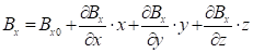
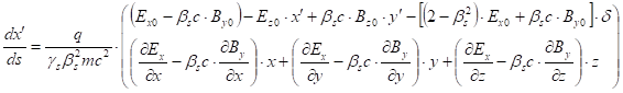
![]()
We used here:
![]() ,
,
![]() ,
,
![]() .
.
Element with symmetry of revolution
Many elements (solenoids, Einzel lenses, RF cavities (DTL, CDC), supra-elliptical, have symmetry of revolution around the beam axis. In this case, the fields are represented in the cylindrical reference: (r, θ, z).
Then: ![]()
Magnetic solenoid
In solenoid we get at the first order:
![]() ,
,
![]() ,
,
![]() ,
,
![]() .
.
The linearized equations of motion become:
![]()
![]()
Electrostatic Einzel lens
In an electrostatic Einzel lens, we get, at the first order:
![]() ,
,
![]() ,
,
![]() ,
,
![]() .
.
The linearized equations of motion become:
![]()
![]()
![]()
In these equations, we must add the variation of the energy of the synchronous particle:
![]() .
.
RF accelerating cavities
In a RF accelerating cavity we get:
![]() ,
,
![]() ,
,
![]() .
.
At the first ordre:
![]() ,
,
![]() ,
,
![]() .
.
In Cartesian coordinates:
![]() ,
,
![]() ,
,
![]() ,
,
![]() .
.
The linearized equations of motion become:
![]() ,
,
![]() ,
,
![]() .
.
Magnetic quad
In a magnetic quad:
![]() ,
, ![]() and
and ![]()
Then:
![]() ,
,
![]() .
.
Electrostatic quad
In an electrostatic quad:
![]() ,
, ![]() and
and ![]()
Then:
![]()
![]()
A high intensity beam can be described as a combination of:
- the central core, very compact and dense, where linear forces are dominant, leaving the emittance unchanged
- the external halo, much less dense, where some particles have been sent after gaining extra energy and where nonlinear forces are dominant, leading to emittance increase.
Let us consider the case of a dense, uniform core where self-forces are strictly linear, surrounded by a non-uniform and very few dense halo. In such a configuration, the corehalo limit is clearly given by the location where the density gradient abruptly changes from small variations in the halo to a very steep (infinite variation when arriving on the “wall” of the core uniform distribution).
For a more realistic distribution presenting a similar topology but where the density gradient continuously varies, the core-halo limit definition can be generalized as the location where there is the steepest density gradient variation, that is where the Laplacian of the density is maximum. In 1D, it corresponds to the second derivative’s maximum (not to be confused with the second derivative’s zero), which is the inflection point. We will take this location of second derivative maximum as the core-halo limit.
2. At a given position
At a given position along the accelerator and for a given coordinate (spatial or momentum), a histogram is calculated, allowing to obtain the beam density profile. From that, first and then second derivatives are calculated. In order to get rid of numerical noises and in the meantime preserving the abrupt variations of the profile that must be detected, smoothing of the original profile is not appropriate. The method of sliding derivative, calculated on the average of 10 points around the point of interest is used instead. As the halo is expected only at the external part of the beam, only positive maximas of the second derivative should be selected (For a constant profile), due to numerical noise, the second derivatives are close to zero but either positive or negative. That is why, only positive maximas that are much bigger (in absolute value than negative minimas should be selected).
That procedure gives core-halo limits that
correspond roughly to what can be seen intuitively when looking at a density
profile. For a Gaussian profile characterised by the standard deviation s, this limit is ![]() . For a pure
square, triangular or parabolic profile, there is no halo as expected.
. For a pure
square, triangular or parabolic profile, there is no halo as expected.
3. Along the accelerator
Once the core-halo limit is determined, the following quantities can be given along the accelerators:
· The core maximum size and the halo maximum size (to be considered instead of the classical beam envelope)
·
The percentage of halo size ![]()
·
The percentage of halo particles ![]()
·
The halo density ![]()
· Percentage of particles initially in the halo; for a given position considered as an initial one, this percentage is 100%, then decreases (while oscillating because of transfer with other planes), indicating the replenishment rate of halo particles.
(Reference: Core-halo issues for a very high intensity beam, P. A. P. Nghiem, N. Chauvin, W. Simeoni Jr., D. Uriot, Applied Physics Letters, 104, 074109 (2014).
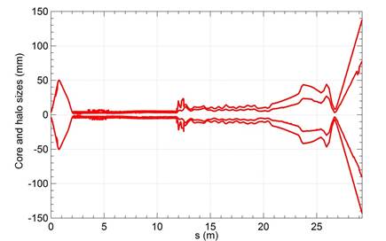
Figure: Core size (internal line and halo size) (external line along the accelerator)
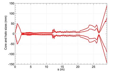
Figure: Percentage of halo size along the accelerator
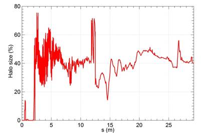
Figure: Percentage of halo particles along the accelerator
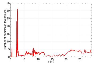
Figure: Halo density along the accelerator
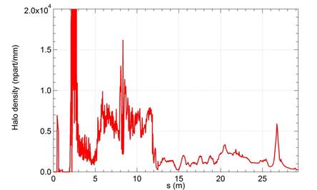
Figure: Percentage of particles initially in the halo along the SRF Linac
(Note written by Ciprian Plostinar
The 3D magnetic field components and their derivates for a multipole magnet in the region close to the axis can be expressed as given by the gradient of a scalar magnetic potential function, V.
The proposed solution in the literature for the scalar potential is of the form:

Where G(z is the magnetic gradient along the longitudinal axis.
More explicitly, for a quadrupole (n=2, the scalar potential is:
![]()
And the three magnetic field components in Cartesian coordinates are given by:
![]()
![]()
![]()
|
DY :
ye -= DY ys += DY
|
|
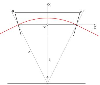
|
DX :
Input drift (DX×sin(θ/2))
Output drift (DX×sin(θ /2))
|
|
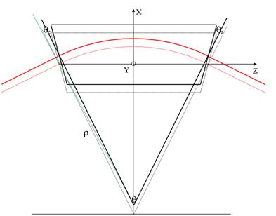
|
DZ :
Input drift (DZ×cos(θ /2)) Output drfit (-DZ×cos(θ/2) ) |
|

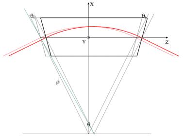
At the input:
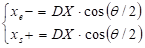
Mθ, the rotation matrix of the dipole (around an axis, meaning given by the law of the corkscrew):
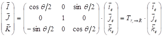

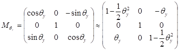
We also gave the second order development of the matrix (be careful, in this case, the determinant is not zero).
The matrix expressing the total rotation of the dipole is the product of the three rotation matrices. However, this product is not commutative.
On the other hand, assuming that the angles of rotation are small and remaining at the second order, we can then find a simplified matrix for the rotation of the elements:

It is this matrix that we will use in PARTRAN. It is obviously approximated, but most certainly less than knowing the magnitude of the errors. Note, however, that its determinant is non-zero (in order 4. The choice of the diagonal is not unique. It is however the one that minimizes the determinant for equal angles of rotation in all directions.
The momemtum ![]() in the fram
in the fram ![]() become then
become then ![]() in the frame
in the frame ![]() :
:
![]() . (1)
. (1)
A particle of coordinates ![]() in the frame
in the frame ![]() centered on E
get then coordinates
centered on E
get then coordinates ![]() in the frame
in the frame ![]() centered on E*
such as :
centered on E*
such as :

l is the half length of the rope at the main path of the magnet.
We get : ![]() .
.
then :
 (2)
(2)
with : ![]() .
.
The input procedure is as follows::
A particle enters the dipole with the coordinates
in the frame ![]() in the frame
in the frame![]() .
.
Its reduced momemtum ![]() in
in ![]() is calculated with
is calculated with![]() .
.
It is then transformed into ![]() with (1), then we
use:
with (1), then we
use: ![]() , …
, …
Its position in frame ![]() i obtained with
(2).
i obtained with
(2).
A drift length ![]() has to be added
in front of the bend matrix.
has to be added
in front of the bend matrix.
The entry corner is treated as a thin lens "like in PARMILA" taking into account the influence of the magnetic leakage field.
The dipole matrix as it was used before is
replaced by a nonlinear transport in the frame![]() . The calculation
is detailed below:
. The calculation
is detailed below:
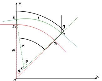
The coordinates of the points are given in the coordinate frame (X, Y) centered on O.
![]() ,
, ![]() ,
, ![]()
The trajectory of the particle is a circle of radius of curvature ρ :
![]()
Find the coordinates of the center of this circle C :
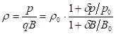
Þ 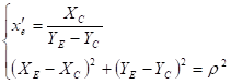
Find the coordinates of the exit position S of the particle:
![]()
Þ 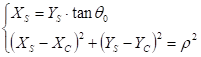
We deduce its exit position, ![]() , of the particle
in the reference frame linked to the reference trajectory:
, of the particle
in the reference frame linked to the reference trajectory:
![]()
![]()
Let us calculate the angle of the particle
at exit in the reference frame linked to the reference trajectory ![]() :
:
![]() ,
,
Þ ![]()
Let us calculate the length of the
trajectory: ![]()
![]()
Þ ![]() .
.
In the vertical plane, the magnet can be considered as a drift:
![]() .
.
Bend output
At the exit of the dipole, the particle is
at the position ![]() .
.
We get:
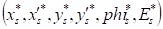
Vector ![]() in the ssytem
in the ssytem ![]() become the
become the ![]() in the frame
in the frame ![]() :
:
![]() . (3)
. (3)
A particle of coordonate ![]() in the frame
in the frame ![]() centered on S*
get then the coodonates
centered on S*
get then the coodonates![]() in the frame
in the frame ![]() centered onré S
such as :
centered onré S
such as :
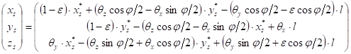 (4)
(4)
then :
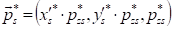 (2)
(2)
with : ![]() .
.
The output procedure is as follows:
A particle leaves the dipole with the
coordinates ![]() in the frame
in the frame ![]() .
.
Its reduced momentum ![]() dans
dans ![]() is calculated
with
is calculated
with ![]() .
.
The it is transformed in ![]() avec (3), then we
take :
avec (3), then we
take : ![]() , …
, …
Its position in the frame ![]() is obtained with
(2).
is obtained with
(2).
A drift lentgh ![]() has to be added.
has to be added.
Some functionalities are available in TraceWin code in order to study the cavity behavior and more generally the linac behavior during the transient time of the cavity RF fields or of the beam current pulse. To have some more details about motivations, objectives and results of this functionality, have a look about the following publication:
Dynamic compensation of an rf cavity failure in a superconducting linac
Jean-Luc Biarrotte and Didier Uriot
PHYSICAL REVIEW SPECIAL TOPICS - ACCELERATORS AND BEAMS 11, 072803 (2008
The spoke and elliptical RF superconducting cavities operate with the TM010-p mode, which produces an accelerating RF voltage on the cavity axis. Using the RLC circuit analogy, the behavior of the “cavity + beam” system can be described to first order by the following equation:
(1 ![]()
![]() represents the
low frequency component of the accelerating voltage created in the cavity at
the operating RF frequency
represents the
low frequency component of the accelerating voltage created in the cavity at
the operating RF frequency ![]() . Its amplitude
. Its amplitude ![]() gives the voltage
seen by a particle, with velocity b and optimal phase, while crossing the
cavity (the Transit Time Factor is included). Its phase
gives the voltage
seen by a particle, with velocity b and optimal phase, while crossing the
cavity (the Transit Time Factor is included). Its phase ![]() gives the phase
of this accelerating voltage, compared to the reference phase of the system
which is chosen here to be the phase giving a 0° synchronous phase. In the case
where the cavities are modeled using punctual gaps, this phase is therefore
directly equal to the synchronous phase.
gives the phase
of this accelerating voltage, compared to the reference phase of the system
which is chosen here to be the phase giving a 0° synchronous phase. In the case
where the cavities are modeled using punctual gaps, this phase is therefore
directly equal to the synchronous phase.
![]() represents the
low frequency component of the beam current crossing the cavity. For short
bunches, its amplitude is given by
represents the
low frequency component of the beam current crossing the cavity. For short
bunches, its amplitude is given by ![]() , where I0
is the beam mean current. Its phase
, where I0
is the beam mean current. Its phase ![]() by definition of
the reference phase.
by definition of
the reference phase.
![]() represents the
low frequency component of the current created by the RF power generator. Its
amplitude is given by
represents the
low frequency component of the current created by the RF power generator. Its
amplitude is given by![]() , where Pinc
is the incident RF power, (r/Q) the cavity shunt impedance (linac
definition), and Qi the incident coupling. Its phase is noted
, where Pinc
is the incident RF power, (r/Q) the cavity shunt impedance (linac
definition), and Qi the incident coupling. Its phase is noted![]() .
.
The resonant frequency of the cavity fcav
is always varying because of various perturbations (microphonics, Lorentz
detuning…, and these perturbations cannot be neglected because of the narrow
bandwidth of the loaded cavity. These fluctuations are included in (1) through
the detuning angle of the cavity,![]() , where QL is the
quality factor of the loaded cavity
, where QL is the
quality factor of the loaded cavity ![]() . We choose to
describe these frequency fluctuations with a first order model using the
following equation (2, where
. We choose to
describe these frequency fluctuations with a first order model using the
following equation (2, where ![]() ,
, ![]() ,
, ![]() are the detuning
contributions from cold tuning system management, Lorentz forces, and
microphonics respectively, kL is the
Lorentz force detuning coefficient in Hz/(MV/m2), and tm is the mechanical time constant of the cavity.
are the detuning
contributions from cold tuning system management, Lorentz forces, and
microphonics respectively, kL is the
Lorentz force detuning coefficient in Hz/(MV/m2), and tm is the mechanical time constant of the cavity.
(2) ![]() with
with ![]()
The solution of the coupled equations (1)
and (2) gives the transient evolution of the accelerating voltage ![]() in the cavity. More
details can be found in.
in the cavity. More
details can be found in.
Due to various perturbations (cavity
frequency variations, beam transients…, the accelerating voltage ![]() produced in the cavity
from (1) + (2) is not stable at all. In order to regulate the accelerating
field and phase, a regulation loop is required, called “Low-level RF” (LLRF)
regulation loop. Its role is to monitor the field produced in the cavity using
a capacitive probe, perform an adequate treatment of the signal, compare it to
the desired (VC, jC) set-point,
and use the detected error to react on the RF high-power amplifier stage via a
PID (Proportional / Integrative / Derivative controller).
produced in the cavity
from (1) + (2) is not stable at all. In order to regulate the accelerating
field and phase, a regulation loop is required, called “Low-level RF” (LLRF)
regulation loop. Its role is to monitor the field produced in the cavity using
a capacitive probe, perform an adequate treatment of the signal, compare it to
the desired (VC, jC) set-point,
and use the detected error to react on the RF high-power amplifier stage via a
PID (Proportional / Integrative / Derivative controller).
A rough but meaningful modeling of such a loop has been defined. The main elements are:
· a comparator that monitors the probe signal and compare it to the desired set-point; at this location of the loop, the signals have been digitalized, and the comparison is made using I/Q signals;
· a PID controller (we will here only use the gain “P” as a first approach);
· a delay or/and a low-pass filter to account for the bandwidth of the whole system; the typical order of magnitude is a few ms delays, and a few kHz cut-off frequency.
The cavity model describing the transient RF cavity behaviour has first been included into the beam envelope and multiparticle TraceWin code and successful validate using tests performed to compare the results produced by this new cavity module with previous Simulink results.
TraceWin code calculates the transport of the reference particle (envelope) or the beam distribution (multiparticle) through the cavities of the linac, and is by default a “static” tool. It has thus been modified to be able to include the “time” variable, and therefore perform simulations at different times. The architecture of the TraceWin code “transient calculation” option is shown in fgure below. Several time steps are involved in the process. From the initial condition, at t=0, where all the cavities are set to their nominal RF fields and phases, different time-based iterations are performed:
every δt0 (time integration step), a new couple of RF field amplitude and phase is evaluated in each cavity of the linac according to RF cavity model; every δt1 (time envelope step), δt1 ³ δt0, a new beam transport calculation is performed through the linac (envelope) transport, using the RF field characteristics (amplitude and phase) obtained at this time in each cavity (which can be modelled either by multi-gap or field map element); this calculation updates the beam characteristics at each linac location; every δt2 (time multiparticle step), δt2 ³ δt1, a multiparticle transport simulation is performed; this calculation updates the beam characteristics at each linac location;
every δt3 (time storage step), δt3 ³ δt2, all the linac and beam characteristics at each location are stored.

Code architecture.
The computation time strongly depends on the choice of these different time steps, and especially on δt1 and δt2; δt3 is fixed by the available memory. Typically, to simulate accurately a 10 ms linac behavior, the time steps are respectively chosen to δt0=1 ns, δt1=1 µs, δt2=10 µs and δt3=10 µs..
Finally, let’s note that for each kind of cavity of the linac, a file has to be created in order to indicate to the transport code its main characteristics. These files have to contain also the feedback loop parameters, which can be different according to the cavity type. Some extra parameters as microphonic frequencies and amplitudes can be added if needed.
Lacc 0.29792 ; Physical accelerating length of the cavity [m]
rsqN 220 ; Optimal shunt impedance [Ω]
rsQ0 4181.98 ; (*)
rsQ1 -81304.21 ; (*)
rsQ2 612270.40 ; (*)
rsQ3 -2303524.54 ; (*)
rsQ4 4695528.24 ; (*)
rsQ5 -4989523.30 ; (*)
rsQ6 2175215.22 ; (*)
Kl -8 ; Lorenz factor [Hz/(MV/m2]
To_m 0.002 ; Cavity mechanical constant
NMIC 0 ; Number of microphonic frequency perturbations to consider
FMIC 100 600 1000 ; List of microphonic frequencies [Hz]
DFMIC 30 10 5 ; List of microphonic amplitudes
Rres 10e-9 ; Niobium surface resistance [Ω]
T 4.2 ; Cryogenic operating temperature [K]
Tc 9.2 ; Nobium critical temperature [K]
G 100 ; Form factor [Ω]
A 0 ; To define Qo as function of accelerating field (**
Qt 1e12 ; Transmit couplage
Time_Start_Cav 0 ; Time [s] when the RF cavity is set on
Time_Stop_Cav 0.005 ; Time [s] when the RF cavity is set off
Time_Start_Beam 0.0 ; Time [s] when the beam pulse is started
Time_Stop_Beam 100.0 ; Time [s] when the beam pulse is stopped
Gain 20 ; Feed-back gain
Freq_BP_loop 10000 ; Low filter frequency cut (Hz)
PowMax 30000 ; Max power from power supply (W)
Retard_Loop 0 ; Feed-back delay (s)
MargeField 0.7 ; field margin, here 70% available
MargePhase 10 ; RF phase margin, here RF phase can be adjusted of +/-10°
Fast_start ; Allow to avoid transient time need to start cavities at t=0
(*) rsQ = rsqN, but if rsqN equal to 0 then
![]()
(**)
![]() , with
, with ![]()
To cancel a line value put ‘;’ at the beginning
In this example (See “HELP“) menu at the top then “Open example files” and open “Cavity_transient” project file, the second spoke cavity failed at 5 ms. The cavity failure parameters is set in “spoke_25MV_failed.cav” file and the nominal cavity is described in the “spoke_25MV_nominal.cav” file.
CAVITY_PARAMETERS spoke_25MV_nominal.cav
FIELD_MAP 100 597.92 -124.88 50 0 1 0 0 spoke_25MV
Cavity parameters file can be applied on FIELD_MAP, NCELLS, GAP elements.
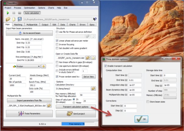
In this box, all the parameters needed to perform the transient simulation have to be set. Don’t forget to “Enable transient simulation”
Simulations can be performed with or without multiparticle option, but in a first time it’s strongly recommended to start only in envelope mode.
Global results can be observe either as a function of the time of the simulation or as at a define time at position elements
The following example shows the beam energy (blue) behavior during the 10 ms of simulation. The first slop at the beginning corresponds to the cavity filling. You can avoid this stage by using the “Fast_start” parameter of the cavity parameters file allowing to start simulation directly at the nominal field in the cavities.
You can see also, starting at 5 ms, the effect of the second cavity failure.
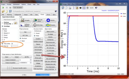
The other possibility is to show the beam behavior at a given time like following example, where at different time the beam envelope is shown. Bellow output beam en energy along the machine at t=3 ms.
Bellow output beam en energy along the machine at t=5.02 ms. The cavity start to failed and the first effects are visible on the output beam.
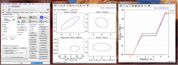
Finally, bellow at 8 ms, almost at the end of the rtransient simulation
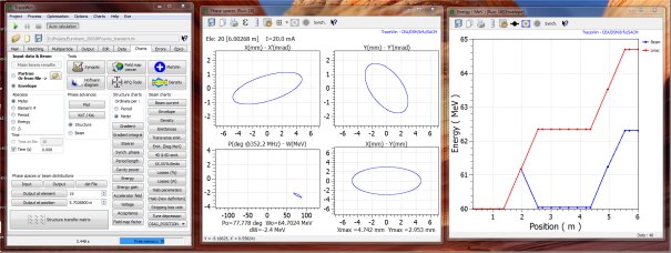
For a time-consuming (purely statistical error study with PARTRAN or Toutatis or envelope), several computers can be used via a client/server architecture (multi-parameter scheme. These remote machines must be running on Window, Linux and MacOS operating systems. You may decide to use these computers only at night or on weekends. You must install and run the "twserver" code on each computer. For each computer, you must choose the number of cores you want to use.
If your simulation is very short (a few seconds), it is probably best to use only your local computer (IP=0.0.0.0) and to choose a number of cores higher than the number of cores actually available. This last point will be determined on a case-by-case basis for your own computer.
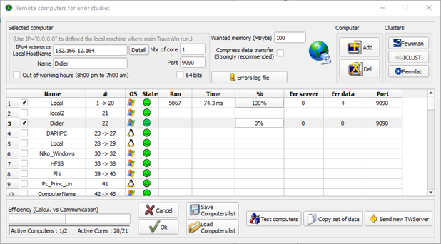
For Windows you need to install “twserver.exe” and for Linux or MacOS install “twserver” code on your remote computers. All you nedd to do is copy the executable file somewhere and launch it. Setup is completely automatic and the final installation will be “C:\TWSever” for Windows and “Home/.TWServer” for Linux or MacOS. Print “./twserver&” for Linux or “twserver.exe” for Windows in a console. All new installation will destroy the running old version and will install the new one in the good directory. Don’t try to start “twserver” directly in its final directory.
Sometime, some remote machines don’t respond to TraceWin requests. There are several reasons for this:
Check your firewall: The TraceWin server needs access to TCP ports (9090 to 9102). Check whether you have selected the "Work only outside working hours" option in the "Remote computer" box management. Also check the minimum memory requirement.
In Windows, the remote server can be disabled locally (right-click) on the icon in the bottom right-hand corner of the system tray. This means that TraceWin will only use this computer when its CPU load is very low.
Before any bug investigation, test all your computers using the "Test computer" button in the "Remote computers" box.
The twserver cannot launch more the N jobs in the same time. N is either defined by default by the number of core available or by the environment variable ‘TWSERVER_N_THREAD=N”. This limitation is only valid for desktop computers and is not used for cluster machines.
Installation on cluster machine.
For CEA Saclay users only:
Download “twserver_without_X” and rename to “twserver. Install “twserver” on the CEA/Irfu clusters named “ISIPIC” or “FEYNMAN”, by starting “twserver” on the master node with the command “./twserver isipic” or “./twserver feynman” depending on the cluster you are on. Set the number of cores you want to use in the “Remote computers” tool in TraceWin.
For ESS cluster users only:
· Download “twserver_without_X” file and copy it to ESS cluster (user@ess01.dcsc.ku.dk).
· Dowload “twservertunnel.sh” file on your computer.
· On cluster:
1. Rename “twserver_without_X” to “twserver”
2. Type “./twserver ess”. This command will install twserver on cluster directory “/data/users/TWServer”. All users must have write and read rights. On the cluster only one occurance of twserve has to run. Each time a new user will type this command the old server will closed and the new one will replace it. (Avoid to do that when twserver is used, you’ll stop a colleague study)
· On your local computer:
1. Type “./twservertunnel open user@ess01.dcsc.ku.dk” This command will create ssh tunnel between your local computer and ESS cluster. It’s necessary because TraceWin communicates to twserver by FTP protocol using port 9090 to 9110 and SFTP is requiered. By this way the port 9090 to 9110 from your local computer will be directly connected to ESS cluster by a ssh tunnel. Unfortunallty for each port (20, you have to type your cluster password. (That can be avoid by creating a ssh key authorization, see your administrator)
2. Launch TraceWin and in remote computer box, add ESS cluster with IP address (127.0.0.1
3. When you want stop your studies don’t forget to closed port tunnels (“./twservertunnel close user@ess01.dcsc.ku.dk”).
· An alternative simpler way is to directly use TraceWin code to ESS cluster (use “TraceWin_libc_2-3-4” version). In this case, after twserver installation you have to add ESS cluster IP to TraceWin remote computer list and you have also to transfer your project data to ESS cluster.
For all other cluster:
First, 3 scripts must be created by the cluster administrator and placed in one of the directories defined in the $PATH variable or the directory where these scripts are located must be added to the $PATH variable.
Then, download the "twserver_without_X" code and rename it to "twserver". Copy "twserver" to the master node of your cluster. Run "./twserver cluster path". A directory "TWServer" will be created in the "path" directory which must already exist and which will host the server itself and all the data necessary to start the various executions as well as all the simulation results. An example of the steps is given below.
Finally, in the TraceWin code, define the number of cores you want to use in the "Remote Computers" tool on the "Errors" page.
· tw_job_run.sh
· tw_job_status.sh
· tw_job_kill.sh
tw_job_run.sh : allows to run an executable with its arguments in the cluster task queue and retry the job ID.
tw_job_status.sh : allows to check the status of a job knowing its ID.
tw_job_kill.sh : allows to cancel a job knowing its ID.
Below is an example of scripts succesufy tested to submit a job to a cluster using the Slurm job scheduler:
All the "echo" lines and their syntax must be scrupulously respected, as they are used for communication with the server.
tw_job_run.sh
#!/bin/sh
# Retrieving the code to run and its 3 arguments
full_name_code=$1
arg1=$2
arg2=$3
arg3=$4
#Launch job with argument en return job id in ID variable
ID=$(sbatch --parsable --ntasks=1 --wrap="$full_name_code $arg1 $arg2 $arg3)"
# syntax to be respected
echo "job# $ID launched"
tw_job_status.sh
#!/bin/sh
# Retrieving the ID of the job passed as an argument
job_id=$1
# Executing the "squeue" command to retrieve the job status
job_status=$(squeue --job $job_id | awk 'NR==2 {print $5})'
# Checking the status of the job to set the return value (3 possible cases)
if [[ "$job_status" == "R" || "$job_status" == "CF" || "$job_status" == "CG" || "$job_status" == "PD" ]]; then
# The job is running or waiting in the queue or other conditions requiring waiting
echo "Job# $job_id status: RUNNING"
elif [[ "$job_status" == "F" || "$job_status" == "E" ]]; then
# The job is in error or any other condition that requires killing it
echo "Job# $job_id status: ERROR"
else
#The job is finished
echo "Job# $job_id status: END"
fi
tw_job_kill.sh
#!/bin/sh
# Retrieving the ID of the job passed as an argument
job_id=$1
# kill the jon number job_id
scancel $job_id
Example of installation procedure:
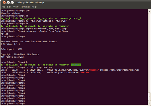
Main configuration
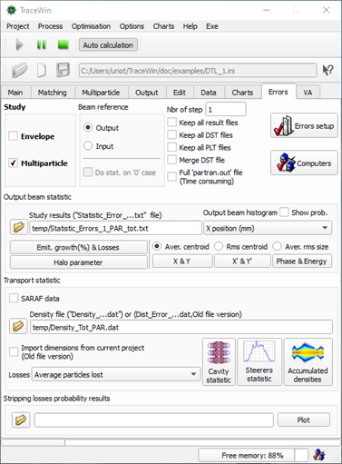
Study (Envelope / Multiparticle: One or both of these options must be selected to allow a statistical or non-statistical error study can be performed at the end of the simulation and tuning process of the linac.
Beam reference (Output / Input: Some output beam statistcs such as beam losses or emittance increases are performed according to a beam reference. If “Output” is selected, the reference run will be the output run obtained by simulating of the perfect machine without errors. In this case, the error study will only start after this reference run (This reference run can be done using the same statistics as the error runs if the "Do stat. On '0' case" option is selected). This allows the static variation of the input distribution to be included as a reference beam.
Number of steps: the error amplitudes defined by the commands (ERROR_...), see below will be applied at 100% or progressively depending on this parameter. '10' means that the error amplitude will be 10% in a first study, then 20% in the second etc... Each of these studies will have associated output files.
Errrors setup: TraceWin allows to study many type of errors. They are divided into two types: “Input beam scan” and the “statistical errors”.
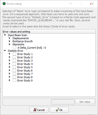
Input beam scan:
The first type concerns the sensitivity of the machine to a variation of the input beam parameters, such as beam displacement, emittance growth, beam mismatch and so on. These scan-based studies require a "Number of steps" parameter greater than 1. For this type of error, the magnitude of the errors have to be defined directly in the interface (see below).
For this type of study, in the "Computer" box, you should select only your local computer (IP:0.0.0.0) with a single core.
Four types of error are available:
- Beam displacement: The beam input position is not centred.
- Emittance growth: The input beam emittance is increased by a percentage.
- Beam mismatch: The input beam is mismatched by a percentage. A 20 % mismatch in X plane means that αx and βx are multiplied by (1.2²).
- Beam Current error: Allows to study the effect of the input beam current variation.
In the example below, if “Nulmber of step” is 10, the input horizontal and vertical beam position of the input beam will move from -10 to 10 in 10 steps. Both error studies will be performed one after the other. At the end, you can view at the results like the output beam behaviour according to the input beam errors by using the two file “X_Displacement_ENV.txt” and “Y_Displacement_ENV.txt” if “Envelope study” is selected or “X_Displacement_PAR.txt” and “Y_Displacement_PAR.txt” if “Multiparticles study” is selected. There are located in the “Calculation directory” defined in the “Main” TraceWin page. One of these files has to be selected in “Studies results” of the “Errors” page.
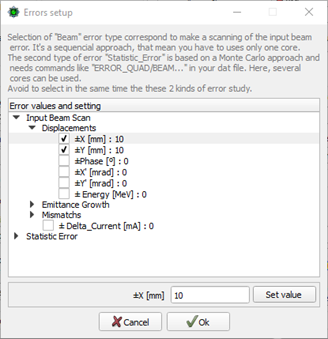
Statistic errors
The second type of error is an statistical studies based on montercalo approach.
The first step is to specified in the structure file which type of error with which amplitude will be applied to the different components of the accelerator (see the help about “ERRRO_xxxx” commands).
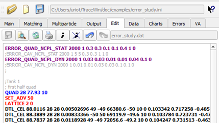
The second step is to define the different failure studies to be performed. Up to 9 can be defined and they are performed sequentially. For each of them, define the element and the error to be considered in the statistical study. Then define the number of runs for the study in question (here: 1000). Note that the total number of runs = "number of steps" x "number of runs". Random errors on the input beam can also be included (select "Input beam") and their amplitudes can be defined using the "ERROR_BEAM" command.
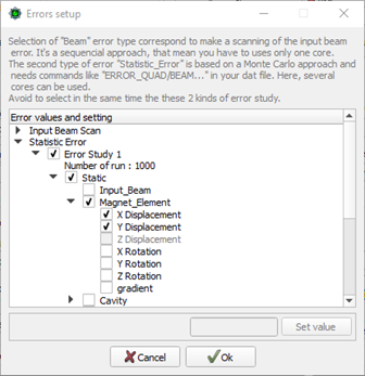
If you have defined a correction scheme in your data file, this scheme will be applied to each machine according to the following procedure:
· Your machine is set with your correction scheme (diagnostics associated with the “ADJUST” command and “Match using diagnostics" selected in the "Matching" page will be the reference machine)
· Random static errors are applied to your linac based on your static error commands.
· Your correction scheme is executed.
· Dynamic random errors are applied to your linac based on your dynamic error commands.
· The final simulation is performed.
Keep all result files: During the single simulation, many files are written, concerning the beam, the transport, tuning. During the error studies, they are concatenated into single files and then deleted, but if this option is selected, they will all be kept (be careful with the final size of the set).
Keep all DST file: Prevents the deletion of all output beam distribution files (*.dst) for each run (be careful with the final size of the set).
MergeDST file: All output beam distribution files (*.dst) are merged into a single dst file. (be careful with the final size and the number of particles will be limited to 2 billion).
Keep all PLT file: Prevents all files containing the beam distribution along the entire structure (*.plt) for each run from being deleted (be careful with the final size of the set).
Full ‘partran.out” file: This file contains all the beam parameters at each position on the machine (see help on this). Normally only the last position is calculated and saved during the error study to save time, unless this option is selected.
Cavity statistic: Tool to visualise the RF field and cavity phase statistics when a cavity tuning scheme is applied to the accelerator structure (see chapter "Cavity tuning").
Steerer statistic: Tool to visualise the steerer strength statistics when an alignment scheme is applied to the accelerator structure.
Accumulated density: Tool to visualise the evolution of the main parameters and the beam distribution projection of the merged beams along the structure.
Losses: Various curves relating to the distribution and probability of beam losses along the structure.
Check an error study configuration:
Before running thousands of simulations, it may be useful to check how the selected errors would look with the amplitude defined for a single simulation. Therefore, set the "Include errors defined in Data N°:" option to "1" on the "Main" page, which will allow you to check for a single simulation the error defined in "Error study: 1" of "Error Settings". To do this, deactivate the "Envelope study" or "Multiparticle study" on the "Errors" page. The random errors and therefore the simulation will always be the same if the seed is frozen, otherwise each new run will be performed with different errors.

In this example (see "Help" menu), "Open examples", "Error_study" project a statistical error study is performed concerning the quadrupole alignment errors in a DTL tank. Quadrupoles misalignment study from 0 mm to 0.3 mm in 10 steps. 20 cores on a local machine are used (about half an hour was needed to complete). On the “Output” page during the error study, beam losses occur from 90% of the maximum error amplitudes.
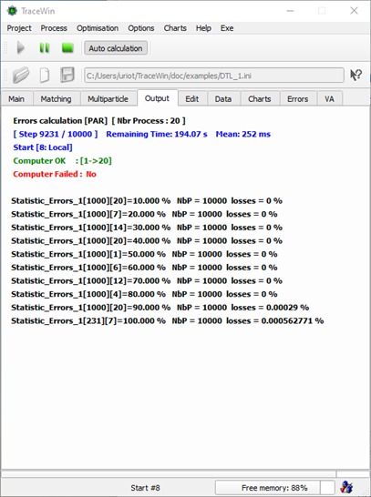
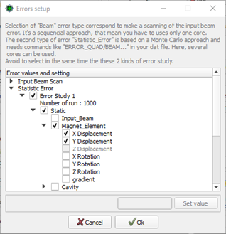
Results (“error_study” project example)

Emit. growth(% & losses) : Losses are observed from 60% of the error, i.e. a misalignment of the order of 1.8 mm. The transverse emittance growths are limited to 14% for 3 mm of error.
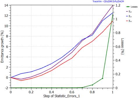
X & Y (rms centroid) : rms output beam centroid grows linearly with the amplitude of the errors, which is expected by the theory.
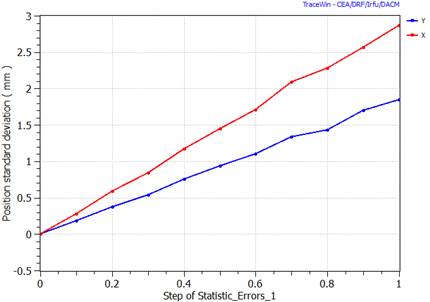
Output beam histogram (X position) : on 1000 runs, the horizontal position of the beam can reach +/- 8 mm.
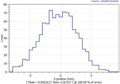
Average power lost : (file: “Density_tot_PAR_1_1.0000.dat”). This file corresponds to error study#1 at case (1.0000 100% error amplitude). We observe the distribution of the average power deposited along the structure.
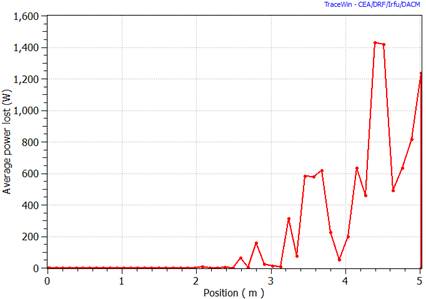
Accumulated density (Density level & X) : (for file: “Density_tot_PAR_1_1.0000.dat”). Shows the particle density probability repartition all along the structure for the 1000 runs of 10000 particles. (10-1 is 90% of the 107 particles, 10-2 is 99% of the 107 particles…)
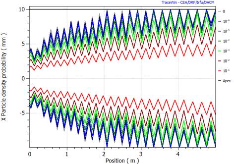
If you want to combine other quadrupole errors, you just have to select them and restart the study. Obviously, cavity errors can be combined with quadrupole error. You could also insert in your data file a scheme of correction; steerers associated with beam monitor positions. Start a new study in order to see if your scheme is efficient.
Results (“error_study2” project example)
In this second example (see "Help" menu), "Open examples", "Error_study2" project a similar statistical error study is performed concerning the quadrupole alignment errors in a DTL tank, but this time including correction scheme. This means that, steerers are included in the structure as well as position diagnostics. On the “Matching” page, the option “Macth using Diagnostics” has to be selected and in this example diagnostics position accuracy is set to 1 mm (see DIAG_POSITION). In order to take this into account in the study, the option "Take into account diagnoctics accuracy" must be selected.
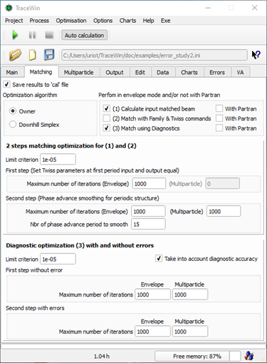
X & Y (rms centroid) : rms output beam centroid is this time smaller than project without correction scheme.
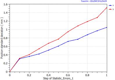
Average power lost : (file: “Density_tot_PAR_1_1.0000.dat”), 100% of error amplitude. Average losses is much lower than project without correction scheme.
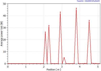
Steerers statistic : This tools from “Errors” page allows to visualize statistic about steerer strength.
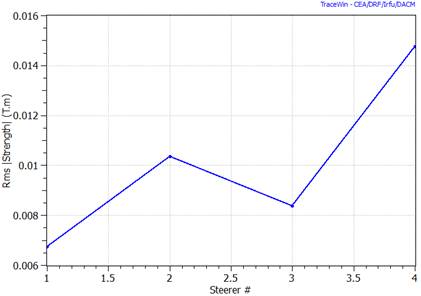
Implementation
Two different approaches to implement the virtual accelerator are possible, either we integrate the simulation model into the control system (like XAL @SNS or J-PARC example or we integrate a part of the control system into the simulation code (like Traxce3D)). This is the last approach which has been developed making the simulation code associated to control system as an independent high level application. The control system was based to EPICS (Experimental Physics and Industrial Control System, as many accelerator in the world).
With EPICS is provided most of the gateways or programming interface to advanced programming languages. The database is accessed through the "Channel Access" protocol. Finally, the graphical user interfaces are various and many. Modern and useful, EPICS seems for the time being the ideal tool to perform this kind of development. Figure 5 represents the architecture of EPICS.
EPICS is based on a data base "EPICS BD" composed of recordings or "RECORD" objects representing equipment. Each of these RECORDs contains many fields representing the main parameters of the equipment. All these information are accessible for reading and writing via the Channel Access.
To simplify, we only considered for given equipment only 3 fields of the RECORD:
• The command: represents the value that we want to order to the equipment. For example, you wish to send 200A in the coil of a solenoid.
• The virtual command: represents the value that we want to order to the code for the simulation of this equipment. For example, you wish to simulate the machine with 200A in the solenoid coil.
• The acquisition: represents the acquisition of the value of this equipment. For example, we measure 200.3 A in the power supply connected to the solenoid.
With the structure of the RECORDs as it is defined in EPCIS, we can use therefore a single database to represent two accelerators. It should be noted that some components such as diagnostics will be used through the last field.
The different fields of the RECORDs are accessed via the 'Real Process Variable' or PV's variable.
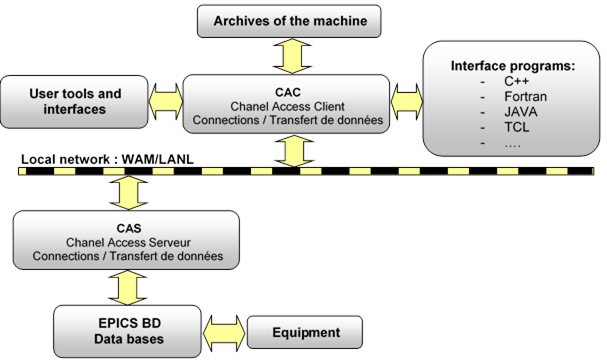
Interface TraceWin « EPICS
The dialogues between TraceWin and EPICS are made through "EPICS Base" library. It is the heart of EPICS, including code sources of the base system or kernel, libraries for interfacing with different operating systems, Channel Access libraries, the standard RECORD and many other tools. Among the different EPICS version, we used the 3.16.0.1. This base allows to build a Chanel Access Client (ACC for reading and writing in the database of EPICS. The process should use a database, to be defined, internal to the simulation code making the correspondences between the syntax and the physical quantities in TraceWin and EPICS such it is described in figure below.
2 versions, named TraceWinVA, have been developed for Windows (64bits) and Linux (64bits) (*). All developments have been done in C++ language and the final architecture is visible below. Both codes are fully stand-alone and don't require external library installation. It is thus very easy to install them, usually the linux version, on a sufficiently powerful computer dedicated to the calculation in accelerator control rooms.
(* If your system requires a 32-bit version, it could be provided only on request).
Even if “TraceWinVA” and “TraceWin” codes seem very similar, it’s not exactly true and we still recommande to use “TraceWin” code for pure simulations because a little bit more efficient.
TraceWinVA is a beta version in even if it contains most of the major features; it is not yet complete and tested.
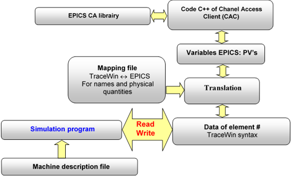
Structure of the code of the virtual accelerator
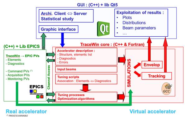
Implementation in TraceWinVA code.
One of the difficulties is the synchronization of the EPCIS commands with the code. In other words, how do you know that a command has gone to EPICS and then check that the concerned equipment has been put to value requested? The example of power supply for magnetic element equipment illustrates this difficulty. Already developed and tested on IPHI and SPIRAL2 projects, both required different approaches to control usual power supply. We considere today that the IPHI method is the most usual way and it’s the default method use in TraceWinVA code, but probbalby new method more efficient could be implemented on another project according to machine specificities.
IPHI (Default)
Figue below presents the algorithm for synchronization of a command dedicated to a power supply of the IPHI injector. It is based on two waiting loops. The first is intended to await the arrival of the command on the equipment while the second waits for stabilization of the acquisition value returned by the power supply to EPCIS data base. That means that the sending of a data speed is therefore linked to the speed of response of the equipment.
Unlike IPHI, power supplies of SPIRAL2 are much more recent and have a flag indicating that they are reaching the final setting. According to this specification a different and more efficient and simple scheme has been developed for SPIRAL2 project.
This example shows that it is not always possible to standardize the code for all equipment and some necessary adaptations for the specific features of the elements of each machine have to be considered and implemented.
|
|
|
|
Writing algorithm for IPHI power supplies |
Writing algorithm for SPIRAL2 power supplies |
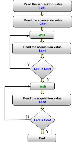
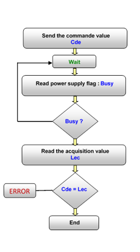
Obviously, in the VA software no waiting loop are used and all PV are monitoring in asynchrony way.
In addition, it is important to match the physical units used in TraceWin and EPICS. For example, TraceWin knows the magnetic field gradient G(T/m) of a quadrupole while EPICS works with the power supply current I(A). This necessarily implies to provide to TraceWinVA the corresponding G(I), see example.
The next is based on the project example named "Virtual_accelerator" from the “Help” menu then “Open examples”.
In TraceWinVA’s tabsheet “Epics”, 3 options are available to control synchronization between the EPICS data base and the simulation code:
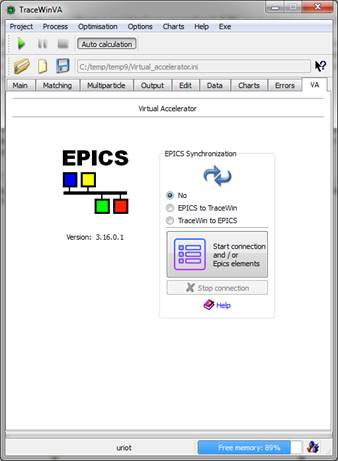
· No : means the code doesn’t provide connection with the EPICS data base.
· EPICS to TraceWin: In this mode, any action on the control system of the machine affects at the same time on the real accelerator and on the virtual one. The virtual Accelerator is directly related to the adjustment of the real machine parameters and simulates it. This simulation can be automatically started at each change of a setting or be done periodically. The machine is under the permanent supervision of the virtual machine.
The diagnostic values resulting from the simulation can be sent to the real machine, allowing the virtual machine to be used to test high-level control command procedures.
· TraceWin to EPICS: The first interest of this mode is its capacity to send the machine setting calculated by the simulation code into control system of the real machine. In this mode, algorithms for automatic adjustment of the simulation code can be used to adjust the real machine. Element setting and daignostics measurement come from real machine. The different procedures of tuning has be defined using DIAG_XXX element and ADJUST commands
You can find in "Help" menu then "Open example", a virtal machine project example.
When a connected mode is selected a button “Stop connection” allows to break this link to come back to an usual standalone simulation code.
Before to select a connection mode, the liste of elements has to be defined using button “Start connection and/or Epics Elements”. It provides the tools allowing to visualize and initialize the common elements defined in TraceWinVA code and in EPICS data base. Fist stage consists to go the the tab-sheet “Epics data”, see below, in order to defined the liste of EPICS elements and their main parameters.
Epics tool – “Epics data”
The page contains all data needed to read and set the elements defined in the EPICS data base, including diagnostics, typically PV names and some other parameters.
- The name of element has to be similar to the name defined in the structure file page.
- G(I) has to be defined either in the GUI and in the structure file using the EXCITATION_CURVE command for magnetic elements.
- Today, recognized elements are only FIELD_MAP, but future extension to usual elements is possible.
- “Precision” parameter has to be chosen very carefully, because it is used to end an EPICS command before the time_out defined by "Time Cde" parameter.
- When you add, delete or change something a reinitialisation is mandatory.
- All data has to be saved in a “*.epics” file.
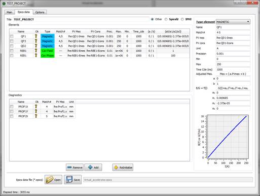
List of elements and diagnostics used from EPICS data base
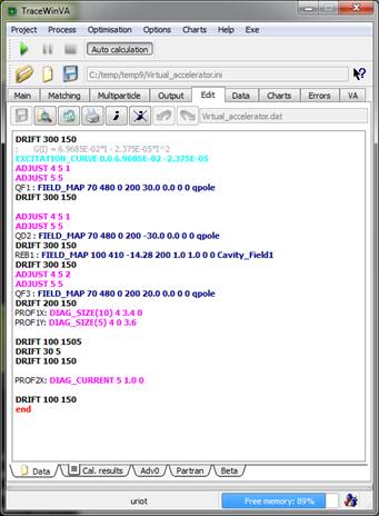
Data file of TraceWin describing the structure of the simulated machine
Epics tool – “Main”
This main page, displays the synchronized PV values defined in the preceding page. All actions in the control system of the machine are automatically visible here. In addition, directly from this page it is possible to modify individually a PV value which causes a direct action on the machine. Only common elements and diagnostics of EPICS tools and structure file are visible on this page. The matching “TraceWin_all” shows all of them. The liste of “Matching TraceWin N°#” correspond to the different matchings defined in the structure file and an optimization can be launched directly on the real machine based on the measurements of the diagnostics.
Button “Set” allows to individually control an element on the real machine and also test the different EPCIS parameters of this element.
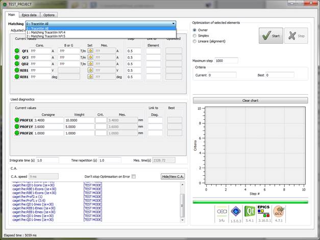
Visualization and monitored elements.
Epics tool – “Options”
Some options are available here; the main one is the “Test mode”. Set by defaut in the example, it allows to simulate a EPICS connection. You have to remove it to really send command to the real machine.
“Number precision” set the number precision in the GUI dispaying.
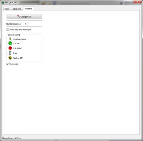
The virtual accelerator program has to be configured in “EPICS to TraceWin” mode. Then all simulation made use the data coming from EPICS data base. As all PVs are monitored and synchronized, when during operation of the real accelerator an element setting is changed in the control system, the simulation is automatically redone and the output charts are refreshed in the same time. In this way, an operator can continuously view the state of the beam and its main parameters wherever it is relevant. A comparison with measurements from diagnostics can thus allow a deep monitoring of the accelerator behavior. A significant discrepancy must alert the operator that something is wrong.
Both figures below show the control room of the IPHI injector before and after an operator has significantly changed a magnetic element of the line. We can immediately see an impact on the envelopes of the beam due to changes in the setting of the machine. Output chart has to set in “Refresh” mode to allow this feature.
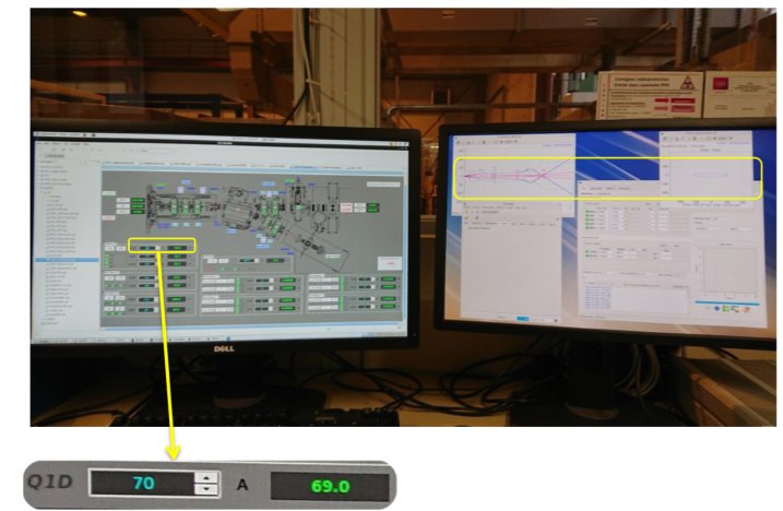
Views of IPHI’s control room, QD1=70A, some outputs of corresponding VA simulation are shown on the right.

Views of IPHI’s control room. QD1 is set by operator to 10A, new VA simulation is launched and new output displays are synchronized.
Quick start from scratch (simple example)
The following example shows how to start step by step a VA configured in EPICS to TraceWin to supervise a simple.lattice including 2 quadripoles, see the image below. The executable to use is 'TraceWinVA'. To simplify, start from the project "Virtual_accelerator.ini" provided in the examples and just change the lattice as below.

The first step is to define the elements before starting the connection with EPICS. The mode must be set to "No" to do this
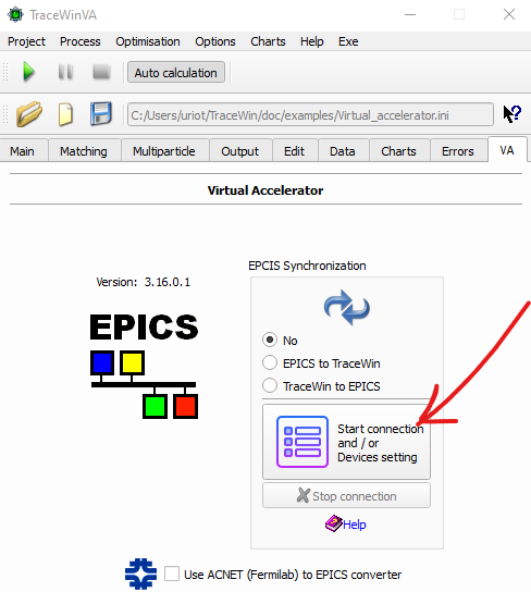
In the "Options" page we will start in "Test mode", thus, no real connection will be made with Epics for the moment but a simulator mode will take over.
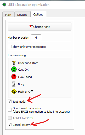
For the first quad you have to fill in, its real characteristics in the machine, the type is MAGNETIC, the parameter 'Name' must be the same as the one defined on the left in the structure file, PV_mes corresponds to Epics PV of the power supply reading, PV_cons is the Epcis PV allowing to control this power supply. The other fields are not determinant except a1 of G(I) which allows to convert A in T/m, here 5 for example. Another possible situation is that there is in the Epics database directly the value of gradient in T/m, in this case put the unit to 'T/m' and a1 to 1
Then add this element using “Add” buton
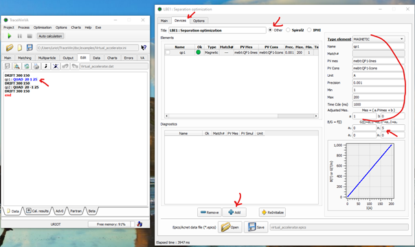
Do the same for the second quadrupole. Then save your configuration, “Save”, and finally reinitialize the configuration, “ReInitialize”
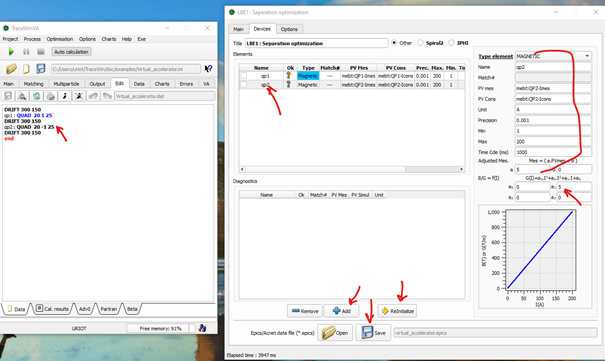
Now you should find in the 'Main' page what is below with the green flag indicating that for the moment the connection is correct (but we are in 'test mode' simulation so it's normal). This simulation will automatically vary the currents to be in dynamic mode as if an operator was doing it on the real machine.
Now we can connect Epics to TraceWin to synchronize the real machine and the simulation (EPICS to TraceWin).
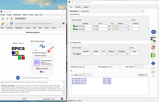
We are configured, launch a simulation, button "Run", display the envelope and press the button of synchonization of the plot (Synch.) Normally here, the envelope evolves with the modification of the currents of the quadrupole power supplies.
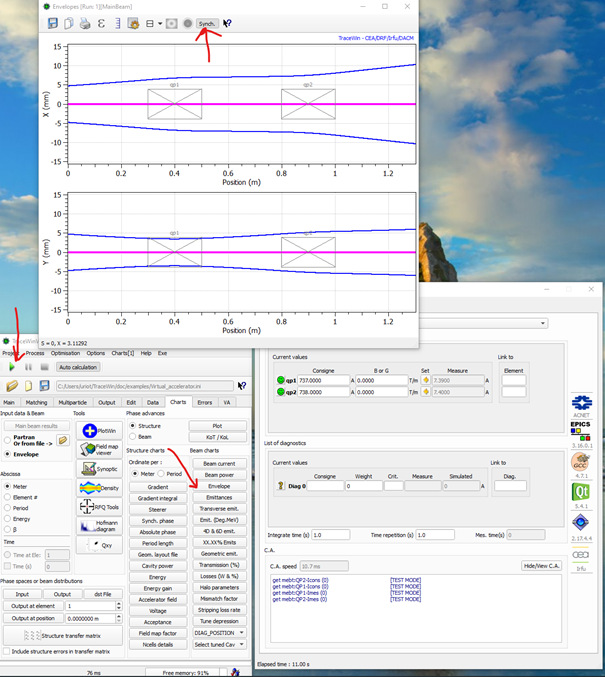
Now stop connection, remove test mode and save the new Epics configuration file.
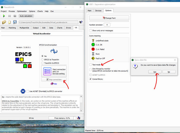
Restart the connection (Start connection) and if your Epcis base is well connected, you will have green flags (in the example below, this is not the case). Then, you can choose EPICS to TraceWin, then launch the simulation and display the plots you want which will be synchronized with the real machine if you press their Sync.button